5.7 Lab: Analyzing experimental data
5.7.1 Study
- Bauer, Paul C., and Bernhard Clemm von Hohenberg. 2020. “Believing and Sharing Information by Fake Sources: An Experiment.” https://doi.org/10.31219/osf.io/mrxvc.
- Abstract: The increasing spread of false stories (“fake news”) represents one of the great challenges digital societies face in the 21st century. A little understood aspect of this phenomenon is why and when people believe the dubious sources behind such news. In a unique survey experiment, we investigate the effect of sources (real vs. fake) and their content (congruent vs. non-congruent with individuals’ attitudes) on belief and sharing. We find that individuals have a higher tendency to believe and a somewhat higher propensity to share news reports by real sources. Our most crucial finding concerns the impact of congruence between reported facts and subjects’ world view. People are more likely to believe a news report by a source that has previously given them congruent information—if the source is a fake source. Machine learning methods used to uncover treatment heterogeneity, highlight that our treatment effects are heterogeneous across values of different covariates such as mainstream media trust or party preference for the AfD. (Bauer and Clemm von Hohenberg 2020)
5.7.2 Data
- Data and files can be directly loaded with the command given below or downloaded from the data folder.
data-randomized-experiments.csv contains a subset of the Bauer and Clemm von Hohenberg (2020) data that we will use for our exercise. We’ll use this data to discuss randomized experiments. The data is based on a survey experiment in which individuals were randomly assigned to two versions of a news report in which only the name of the source (and the design) was varied (The real experiment is a bit more complex). Most variables have two versions where one contains numeric values (_num) and the other one contains labels where it makes sense (_fac). Analogue to our theoretical sessions treatment variables are generally named d_..., outcome variables y_... and covariates x_....
d_treatment_source: Treatment variable where 0 = report is by fake source Nachrichten 360 and 1 = report by real source Tagesschauy_belief_report_*: Outcome scale whether (0-6) measuring belief in truth of report29y_share_report_*: Outcome scales (0,1) measuring whether someone would share the report on different platformsx_age: Gender (Male = 1, Female = 0)x_sex_*: Gender (Male = 1, Female = 0)x_income_*: Income levels (1-11)x_education*: Levels of education (0-5)
For illustration you find an example of the news report and the designs for the source treatment (fake vs. real source) [no need to understand the texts]:

Screenshot of new report


5.7.3 Summary Statistics
Below summary statistics of the data. Table 5.1 displays the summary stats for the nummeric variables, Table 5.2 for the categorical variables.
- Rule: Always provide summary statistics for all variables used in an analysis (e.g., in an appendix) (Why?)
| Statistic | N | Mean | St. Dev. | Min | Max |
| y_belief_report_num | 1,979 | 3.46 | 1.57 | 0.00 | 6.00 |
| y_share_report_email_num | 1,930 | 0.05 | 0.23 | 0.00 | 1.00 |
| y_share_report_fb_num | 1,210 | 0.11 | 0.31 | 0.00 | 1.00 |
| y_share_report_twitter_num | 292 | 0.13 | 0.33 | 0.00 | 1.00 |
| y_share_report_whatsapp_num | 1,639 | 0.09 | 0.28 | 0.00 | 1.00 |
| d_treatment_source | 1,980 | 0.49 | 0.50 | 0 | 1 |
| x_age | 1,980 | 46.53 | 16.07 | 18 | 89 |
| Variable | Distribution |
|---|---|
| Education (German school types) | |
| Abitur | 384 (19) |
| Fach- or Hochschulstudium | 488 (25) |
| Fachhochschulreife | 160 (8) |
| Finished Grundschule | 15 (1) |
| Mittlere Reife, Realschulabschluss, Fachoberschulreife | 673 (34) |
| None | 3 (0) |
| Volks- oder Hauptschulabschluss | 257 (13) |
| Income | |
| 0 to 500€ | 72 (4) |
| 1,001 to 1,500€ | 228 (12) |
| 1,501 to 2,000€ | 244 (12) |
| 2,001 to 2,500€ | 292 (15) |
| 2,501 to 3,000€ | 249 (13) |
| 3,001 to 3,500€ | 213 (11) |
| 3,501 to 4,000€ | 165 (8) |
| 4,001 to 4,500€ | 108 (5) |
| 4,501 to 5,000€ | 92 (5) |
| 5,001€ or more | 137 (7) |
| 501 to 1,000€ | 164 (8) |
| Unknown | 16/1,980 (1) |
5.7.4 Analysis
Analyzing data that comes from a randomized experiment is fairly simple. Given that our assumptions hold (independence, sutva etc.) we can simply compare the average outcome in treatment and control, e.g., with a t-test. See the simple code for one outcome below:
# Import data
  data <- readr::read_csv(sprintf("https://docs.google.com/uc?id=%s&export=download", "1y-TOospohZQevSL1RtFuVEdBaiunyvlh"))


# For a single outcome variable
  t.test(y_belief_report_num ~ d_treatment_source, # ttest for outcomes
         data = data,
         na.action = "na.omit", # omit missings
         var.equal = TRUE) # see ?t.test
##
## Two Sample t-test
##
## data: y_belief_report_num by d_treatment_source
## t = -9.021, df = 1977, p-value < 2.2e-16
## alternative hypothesis: true difference in means is not equal to 0
## 95 percent confidence interval:
## -0.7591045 -0.4879874
## sample estimates:
## mean in group 0 mean in group 1
## 3.153314 3.776860The output indicates that there is indeed a significant difference between the two groups, i.e., that the H0 namely that the difference is equal to 0 can be rejected. Additionally, the difference in the outcome between treatment and control seems substantively large enough. The broom::tidy() function provides easy access to the components of the t-test, simply by wrapping the function broom::tidy(t.test(...)).
Since we have several outcomes we’ll conduct those t-tests using a dplyr pipeline and write the results directly to a table namely Table 5.3.
ttest_results <-
  data %>%
  dplyr::select(d_treatment_source, # select relevant variables
                y_belief_report_num,
                y_share_report_email_num,
                y_share_report_fb_num) %>%
  gather(variable, # write into longformat
         value,
         y_belief_report_num:y_share_report_fb_num) %>%
  group_by(variable) %>% # group by outcome
  do(broom::tidy(t.test(value ~ d_treatment_source, # ttest for outcomes
                 data = .,
                 na.action = "na.omit", # omit missings
                 var.equal = TRUE))) %>%
  ungroup() %>% # ungroup data
  mutate(estimate = estimate2 - estimate1) %>% # Calc. difference
  mutate(estimate = round(estimate, 2)) %>% # Round values
  mutate(p.value = format(round(p.value, 2), nsmall = 2)) %>% # Format
  # Rename outcome variables
  mutate(variable = case_when(variable == "y_belief_report_num" ~ "Belief",
                              variable == "y_share_report_email_num" ~ "Email",
                              variable == "y_share_report_fb_num" ~ "Facebook")) %>%
  mutate(N = parameter + 2) %>% # Why +?
  mutate_if(is.numeric, ~round(., 2)) # Round numeric columsn for display

# Rmarkdown output
  kable(ttest_results,
      caption = "Results for t-tests") %>%
kable_styling(font_size = 12)| variable | estimate1 | estimate2 | statistic | p.value | parameter | conf.low | conf.high | method | alternative | estimate | N |
|---|---|---|---|---|---|---|---|---|---|---|---|
| Belief | 3.15 | 3.78 | -9.02 | 0.00 | 1977 | -0.76 | -0.49 | Two Sample t-test | two.sided | 0.62 | 1979 |
| 0.05 | 0.06 | -1.83 | 0.07 | 1928 | -0.04 | 0.00 | Two Sample t-test | two.sided | 0.02 | 1930 | |
| 0.08 | 0.14 | -2.82 | 0.00 | 1208 | -0.09 | -0.02 | Two Sample t-test | two.sided | 0.05 | 1210 |
If we want to add the difference, i.e., the estimate of the treatment effect to this table we can simply add a column: ttest_results %>% mutate(treatment_effect = estimate2 - estimate1).
Potentially, we may also be keen on visualizing the results. Below in Figure 5.1 we visualize the result for one of our outcomes with ggplot2. In principle, we can make such graphs more informative by adding information and we would probably visually compare the results for our different outcomes (Figure 3, p.11 in Bauer and Clemm von Hohenberg 2020 provides an example).
# Produce the data for the plot
  data_plot <- data %>%
    group_by(d_treatment_source) %>%
    dplyr::select(y_belief_report_num) %>%
    group_by(n_rows = n(), add = TRUE) %>% # Add number of rows
    summarize_all(funs(mean, var, sd, n_na = sum(is.na(.))), na.rm = TRUE) %>%
    mutate(n = n_rows - n_na) %>% # calculate real N # Q: Why do we do that?
    mutate(se = sqrt(var/n),
           ci.error = qt(0.975,df=n-1)*sd/sqrt(n),
           conf.low = mean - ci.error,
           conf.high = mean + ci.error) %>%
    mutate(Group = ifelse(d_treatment_source == 1, "Tagesschau", "Nachrichten 360")) %>%
    mutate(outcome = "Belief") %>%
    mutate(outcome = str_to_title(outcome)) # NOT NECESSARY HERE!

# Plot the data with ggplot
  ggplot(data_plot, aes(x=outcome,  # Setup plot
                        y=mean,
                        group=as.factor(d_treatment_source),
                        color=as.factor(d_treatment_source))) +
      geom_point(position = position_dodge(0.4), size = 1.1) + # Add points
      geom_errorbar(aes(ymin = conf.low, ymax = conf.high), width=.3, # Add errorbar
                     position = position_dodge(0.4), size = 0.7) +
    labs(title = "(A) Outcome: Belief ", # Add lables
         x = "",
         y = "Belief Report 1 (0-6)") +
    scale_color_manual(values=c('red','blue'), # Add/modify legend
                       labels = c("Nachrichten 360 (fake)", "Tagesschau (real)"),
                       name = "Source treatment:")+
    theme_light() + # Choose theme
    theme(panel.grid.major.x = element_blank()) +
    ylim(0, 6)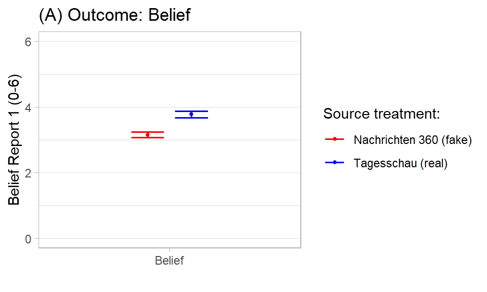
Figure 5.1: Source treatment trust and belief
Other than t-tests we could also estimate linear models (OLS) regressing our outcomes on the treatment variable. In Table 5.4 we do so for 3 outcomes (out of 5).
# LMs
  m1 <- lm(y_belief_report_num ~ d_treatment_source, data = data)
  m2 <- lm(y_share_report_email_num ~ d_treatment_source, data = data)
  m3 <-  lm(y_share_report_fb_num ~d_treatment_source, data = data)


# Produce table
    stargazer::stargazer(m1, m2, m3,
                         summary = TRUE,
                         type="html",
                         font.size="scriptsize",
                         table.placement="H",
                         column.sep.width = "1pt",
                         title = "(#tab:randomization15)Results: Source treatment, belief and sharing intentions",
                         dep.var.labels.include = FALSE,
                         column.labels = c("Belief", "Sharing Email", "Sharing Facebook"),
                         covariate.labels = c("Treatment: Source"),
digits = 2)| Dependent variable: | |||
| Belief | Sharing Email | Sharing Facebook | |
| (1) | (2) | (3) | |
| Treatment: Source | 0.62*** | 0.02* | 0.05*** |
| (0.07) | (0.01) | (0.02) | |
| Constant | 3.15*** | 0.05*** | 0.08*** |
| (0.05) | (0.01) | (0.01) | |
| Observations | 1,979 | 1,930 | 1,210 |
| R2 | 0.04 | 0.002 | 0.01 |
| Adjusted R2 | 0.04 | 0.001 | 0.01 |
| Residual Std. Error | 1.54 (df = 1977) | 0.23 (df = 1928) | 0.31 (df = 1208) |
| F Statistic | 81.38*** (df = 1; 1977) | 3.35* (df = 1; 1928) | 7.93*** (df = 1; 1208) |
| Note: | p<0.1; p<0.05; p<0.01 | ||
Check out ?stargazer for the various stargazer output options.
Finally, we should always provide balance statistics indicating whether treatment and control group are balanced in terms of covariates (when we randomize this should be the case). In essence, we would simply provide statistics of our covariates in treatment and control, e.g., the average as depicted in Table 5.5. In the case of categorical variables one would provide proportions of categories both within the treatment and control groups. Additonally, one may provide statistical tests for those differences (e.g., a t-test comparing the covariate averages between treatment and control) and visualize covariates distributions of units in the treatment and control group.
data_table <- data %>%
            mutate(n_rows = n()) %>% # Add number of rows
            group_by(d_treatment_source) %>% # Group by treatment
            summarise(mean_sex = mean(x_sex_num,  na.rm = TRUE), # Calc. averages
                mean_age = mean(x_age,  na.rm = TRUE),
                n_rows_group = n(),
                n_rows = mean(n_rows),
                n_percent = n_rows_group/n_rows*100) %>%
            dplyr::select(-n_rows) %>%
            mutate_if(is.numeric, round, 2)


knitr::kable(data_table,
             caption = 'Balance statistics',
             format = "html") %>%
kable_styling(full_width = T, font_size = 12) | d_treatment_source | mean_sex | mean_age | n_rows_group | n_percent |
|---|---|---|---|---|
| 0 | 0.51 | 47.15 | 1011 | 51.06 |
| 1 | 0.47 | 45.89 | 969 | 48.94 |
References
Bauer, Paul C, and Bernhard Clemm von Hohenberg. 2020. “Believing and Sharing Information by Fake Sources: An Experiment.”
“On a scale from 0 to 6, do you think that the information in the text of [source] is true? 0 means not at all, 6 means completely”.↩