10.5 Lab
10.5.1 Study
- Minimum wages and employment: A case study of the fast food industry in New Jersey and Pennsylvania (Card and Krueger 1994)
- “On April 1, 1992, New Jersey’s minimum wage rose from $4.25 to $5.05 per hour. To evaluate the impact of the law we surveyed 410 fast-food restaurants in New Jersey and eastern Pennsylvania before and after the rise. Comparisons of employment growth at stores in New Jersey and Pennsylvania (where the minimum wage was constant) provide simple estimates of the effect of the higher minimum wage. We also compare employment changes at stores in New Jersey that were initially paying high wages (above $5) to the changes at lower-wage stores. We find no indication that the rise in the minimum wage reduced employment.”
- Comment (Neumark and Wascher 2000)
- Reconciling the evidence of Card and Krueger (1994) and Neumark and Wascher (2000) (Ropponen 2011)
- Another summary here.
- Treatment: Change in minimum wage (4.25 to 5.05) on April 1, 1992 (in New Jersey)
- Outcome: Employment
- Identification strategy: Difference-in-differences
- For me this study is also a prime example in terms of presenting results (published 1994!)
10.5.2 Visualization of data
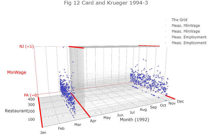
- See a visualization of the data here [Choose Fig 10 on the left.]
10.5.3 Data
- Data and files available under the link given in Section 1.3.
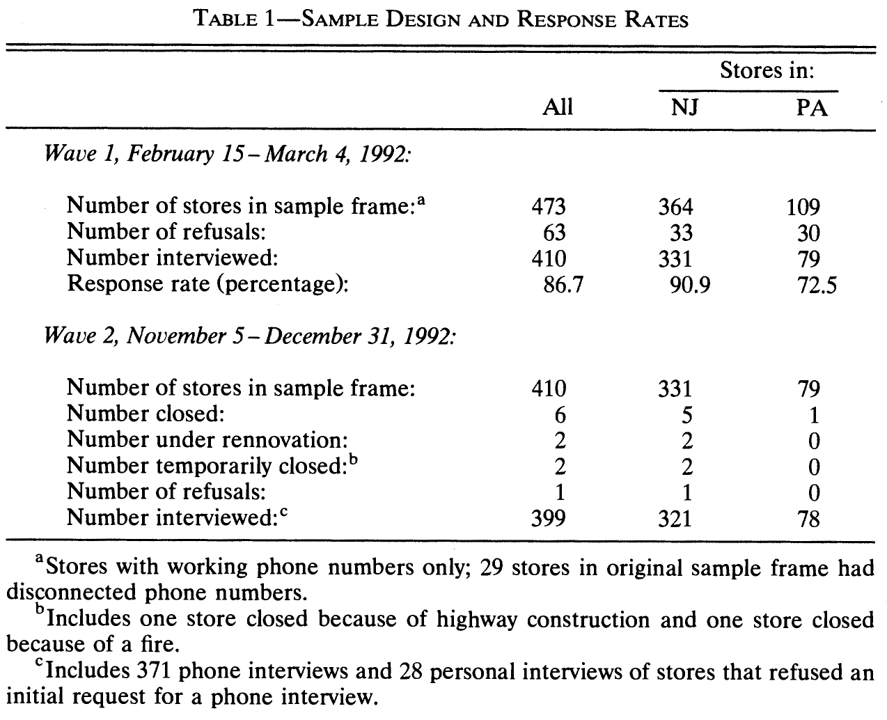
The data data-difference-in-differences.csv is based on the original data provided by Card and Krueger (1994). The original data public.dat and can be downloaded at the MHE Data Archive and there are some R reproduction files provides by Ropponen (2011). Variables have been renamed to decrease cognitive load. Rows are 410 fast-food restaurants in New Jersey and eastern Pennsylvania, interviewed in February/March 1992 and November/December 1992 (see Card and Krueger 1994, Tab. 1, p. 774). The table below provides summary statistics. Analogue to our theoretical sessions treatment variables are generally named d_..., outcome variables y_... and covariates x_....
Below variables that are in the example dataset (I renamed them for convenience).
y_ft_employment_before: Full time equivalent employment before treatment [Outcome]y_ft_employment_after: Full time equivalent employment after treatment [Outcome]d_nj: 1 if New Jersey; 0 if Pennsylvania (treatment variable) [Treatment]x_co_owned: If owned by company = 1x_southern_nj: If in southern NJ = 1x_central_nj: If if in central NJ = 1x_northeast_philadelphia: If in Pennsylvania, northeast suburbs of Philadelphia = 1x_easton_philadelphia: If in Pennsylvania, Easton = 1x_st_wage_before: Starting wage ($/hr) before treatmentx_st_wage_after: Starting wage ($/hr) after treatmentx_burgerking: If Burgerking = 1x_kfc: If KFC = 1x_roys: If Roys = 1x_wendys: If Wendys = 1x_closed_permanently: Closed permanently after treatment
10.5.4 R Code
Below summary statistics of the data.
# Directly import data from shared google folder into R
  data <- readr::read_csv("https://docs.google.com/uc?id=10h_5og14wbNHU-lapQaS1W6SBdzI7W6Z&export=download")
  # Or download and import: data <- readr::read_csv("data-difference-in-differences.csv")
stargazer(data.frame(data), type = "html", summary = TRUE, out = "./www/public.html")| Statistic | N | Mean | St. Dev. | Min | Pctl(25) | Pctl(75) | Max |
| x_co_owned | 410 | 0.344 | 0.476 | 0 | 0 | 1 | 1 |
| x_southern_nj | 410 | 0.227 | 0.419 | 0 | 0 | 0 | 1 |
| x_central_nj | 410 | 0.154 | 0.361 | 0 | 0 | 0 | 1 |
| x_northeast_philadelphia | 410 | 0.088 | 0.283 | 0 | 0 | 0 | 1 |
| x_easton_philadelphia | 410 | 0.105 | 0.307 | 0 | 0 | 0 | 1 |
| x_st_wage_before | 390 | 4.616 | 0.347 | 4.250 | 4.250 | 4.950 | 5.750 |
| x_st_wage_after | 389 | 4.996 | 0.253 | 4.250 | 5.050 | 5.050 | 6.250 |
| x_hrs_open_weekday_before | 410 | 14.439 | 2.810 | 7.000 | 12.000 | 16.000 | 24.000 |
| x_hrs_open_weekday_after | 399 | 14.466 | 2.752 | 8.000 | 12.000 | 16.000 | 24.000 |
| y_ft_employment_before | 398 | 20.999 | 9.750 | 5.000 | 14.562 | 24.500 | 85.000 |
| y_ft_employment_after | 396 | 21.054 | 9.094 | 0.000 | 14.500 | 26.500 | 60.500 |
| d_nj | 410 | 0.807 | 0.395 | 0 | 1 | 1 | 1 |
| d_pa | 410 | 0.193 | 0.395 | 0 | 0 | 0 | 1 |
| x_burgerking | 410 | 0.417 | 0.494 | 0 | 0 | 1 | 1 |
| x_kfc | 410 | 0.195 | 0.397 | 0 | 0 | 0 | 1 |
| x_roys | 410 | 0.241 | 0.428 | 0 | 0 | 0 | 1 |
| x_wendys | 410 | 0.146 | 0.354 | 0 | 0 | 0 | 1 |
| x_closed_permanently | 410 | 0.015 | 0.120 | 0 | 0 | 0 | 1 |
10.5.5 Figure 1 and 2
We start by ‘reproducing’ Figure 1 (p.777) that you see below.
Q: What does the Figure display and what do the authors want to show (discuss with your neighbor)?
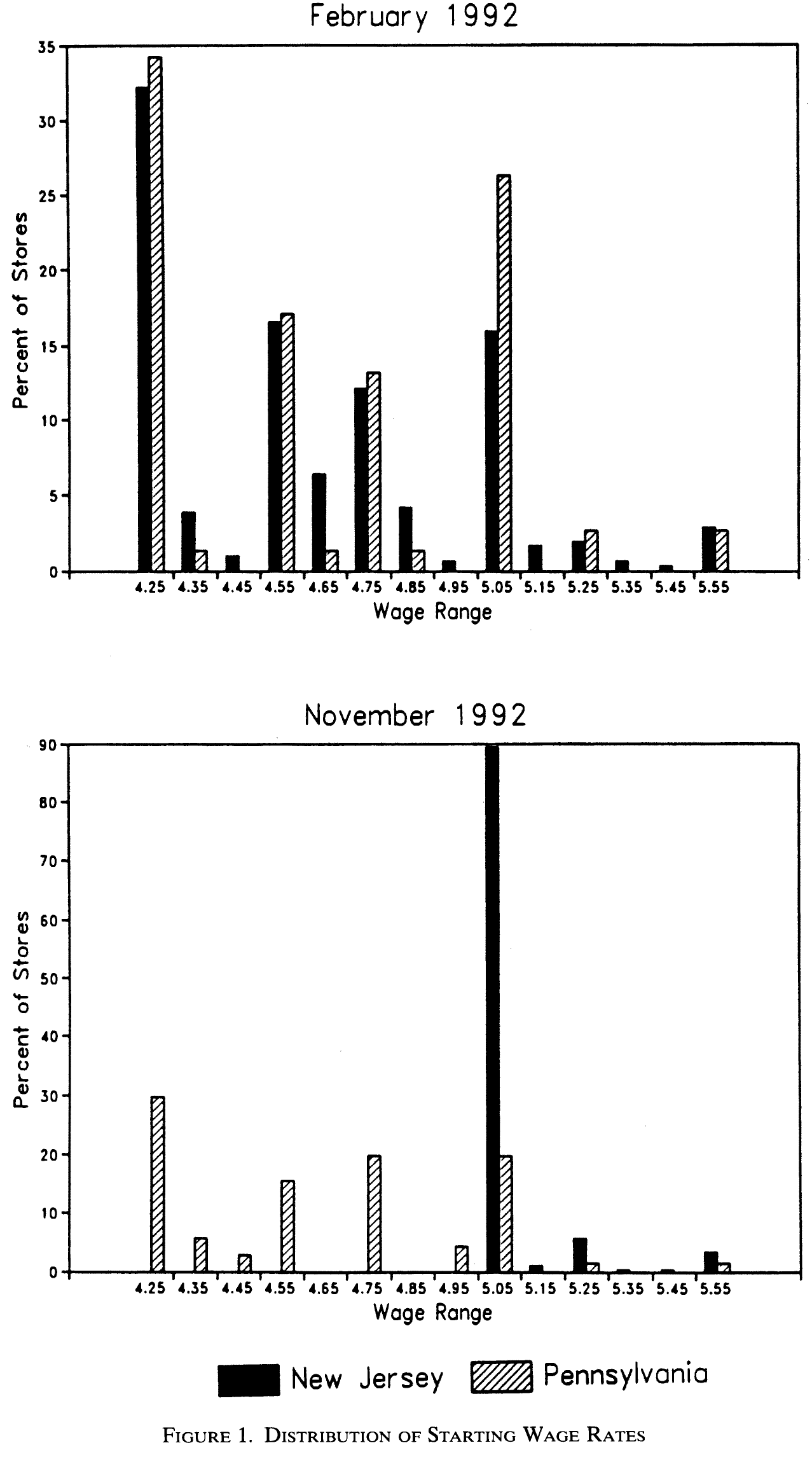
We can reproduce these graphs in R as follows (see Figure 10.1 and Figure 10.2):
#FIGURE 1
  x_st_wage_before_nj <-
  data$x_st_wage_before[data$d_nj == 1]
  x_st_wage_before_pa <-
    data$x_st_wage_before[data$d_pa == 1]

# Make a stacked bar plot - Plotly
# Set histogram bins
  xbins <- list(start=4.20, end=5.60, size=0.1)

# Plotly histogram
  p <- plot_ly(alpha = 0.6) %>%
    add_histogram(x = x_st_wage_before_nj,
                  xbins = xbins,
                  histnorm = "percent",
                  name = "Wage Before (New Jersey)") %>%
    add_histogram(x = x_st_wage_before_pa,
                  xbins = xbins,
                  histnorm = "percent",
                  name = "Wage Before (Pennsylvania)") %>%
    layout(barmode = "group", title = "February 1992",
           xaxis = list(tickvals=seq(4.25, 5.55, 0.1),
                        title = "Wage in $ per hour"),
           yaxis = list(range = c(0, 50)),
                      margin = list(b = 100,
                          l = 80,
                          r = 80,
                          t = 80,
                          pad = 0,
                          autoexpand = TRUE))
  p
Figure 10.1: Wage distribution in February 1992
# WAGE AFTEER
  x_st_wage_after_nj <-
  data$x_st_wage_after[data$d_nj == 1]
  x_st_wage_after_pa <-
    data$x_st_wage_after[data$d_pa == 1]

# Make a stacked bar plot - Plotly
  xbins <- list(start=4.20,
                end=5.60,
                size=0.1)
  p <- plot_ly(alpha = 0.6) %>%
    add_histogram(x = x_st_wage_after_nj,
                  xbins = xbins,
                  histnorm = "percent",
                  name = "Wage After (New Jersey)") %>%
    add_histogram(x = x_st_wage_after_pa,
                  xbins = xbins,
                  histnorm = "percent",
                  , name = "Wage After (Pennsylvania)") %>%
    layout(barmode = "group", title = "November 1992",
           xaxis = list(tickvals=seq(4.25, 5.55, 0.1),
                        title = "Wage in $ per hour"),
             yaxis = list(range = c(0, 100)),
           margin = list(b = 100,
                          l = 80,
                          r = 80,
                          t = 80,
                          pad = 0,
                          autoexpand = TRUE))
  p
Figure 10.2: Wage distribution in November 1992
10.5.6 Table 3
Let’s have a look at Table 3 (p.780). Basically, the table presents mean comparisons of our outcome variable - measure at t0, t1 and the change between t0 and t1 - that we can reproduce.

# Table 3: Column 1-3, Row 1 (from left to right)

# 1st row: MEANs and SEs across subgroups
  results <- data %>% group_by(d_nj) %>% # group_by the treatment variable
            dplyr::select(d_nj, y_ft_employment_before) %>% # only keep variabel of interest
            group_by(N = n(), add = TRUE) %>% # count number of rows
            summarize_all(funs(mean, var, na_sum = sum(is.na(.))), na.rm = TRUE) %>% # aggregate/summarize data
            mutate(n = N - na_sum) %>%
            mutate(se = sqrt(var/n))

# Add row with differences
  results <- bind_rows(results, results[2,]-results[1,])
  results$group<- c("Control (Pennsylvania)", "Treatment (New Jersey)", "Difference")
kable(results, digits=2)| d_nj | N | mean | var | na_sum | n | se | group |
|---|---|---|---|---|---|---|---|
| 0 | 79 | 23.33 | 140.57 | 2 | 77 | 1.35 | Control (Pennsylvania) |
| 1 | 331 | 20.44 | 82.92 | 10 | 321 | 0.51 | Treatment (New Jersey) |
| 1 | 252 | -2.89 | -57.65 | 8 | 244 | -0.84 | Difference |
# Calculate SE for difference: SE = SQR(VAR/N + VAR/N)
  diff_se <- sqrt(results$var[1]/results$n[1] + results$var[2]/results$n[2])
  diff_se
## [1] 1.443583Now it’s your turn… calculate the values for row 2 and row 3, i.e., y_ft_employment_after. Example code below..
# 2nd row: MEANs, SEs etc.
   results <- data %>% group_by(d_nj) %>% # group_by the treatment variable
            dplyr::select(d_nj, ...) %>% # only keep variabel of interest
            group_by(N = n(), add = TRUE) %>% # count number of rows
            summarize_all(funs(mean, var, na_sum = sum(is.na(.))), na.rm = TRUE) %>% # aggregate/summarize data
            mutate(n = N - na_sum) %>%
            mutate(se = sqrt(var/n))


# 3rd row
A slightly different approach using dplyr…
data %>% group_by(d_nj) %>%
  summarise(mean.before = mean(y_ft_employment_before, na.rm=TRUE),
            mean.after = mean(y_ft_employment_after, na.rm=TRUE),
            var.before = var(y_ft_employment_before, na.rm=TRUE),
            var.after = var(y_ft_employment_after, na.rm=TRUE),
            n.before = sum(!is.na(y_ft_employment_before)),
            n.after = sum(!is.na(y_ft_employment_after))) %>%
                mutate(se.mean.before = sqrt(var.before/n.before)) %>%
mutate(se.mean.after = sqrt(var.after/n.after))| d_nj | mean.before | mean.after | var.before | var.after | n.before | n.after | se.mean.before | se.mean.after |
|---|---|---|---|---|---|---|---|---|
| 0 | 23.33117 | 21.16558 | 140.57145 | 68.50429 | 77 | 77 | 1.3511489 | 0.9432212 |
| 1 | 20.43941 | 21.02743 | 82.92359 | 86.36029 | 321 | 319 | 0.5082607 | 0.5203094 |
In Table 4, Row 4 the authors rely on a balanced sample of stores. Q: What is meant by that?
# 4th row: Balanced sample of stores
  # How can I get the stores that have data in both waves?
    df %>% na.omit

    # Filter complete cases across all columns
    data %>% filter(complete.cases(.))

    # Filter complete cases across those two variables
    data %>% filter(complete.cases(y_ft_employment_after,
                                y_ft_employment_before))
10.5.7 Table 4
First we select the data for analysis..
  data2 <- dplyr::select(data,
                         y_ft_employment_after,
                         y_ft_employment_before,
                         d_nj,
                         x_burgerking,
                         x_kfc,
                         x_roys,
                         x_co_owned,
                         x_st_wage_before,
                         x_st_wage_after,
                         x_closed_permanently,
                         x_southern_nj,
                         x_central_nj,
                         x_northeast_philadelphia,
                         x_easton_philadelphia) %>%
           mutate(x_st_wage_after = case_when(x_closed_permanently == 1 ~ NA_character_, # these stores get an NA
                                              TRUE ~ as.character(x_st_wage_after)),
                  x_st_wage_after = as.numeric(x_st_wage_after)) %>%
                  na.omit()
In Table 4 (p. 780) Card & Krueger control for some covariates. Check out the table notes of the table. Remember to always provide the number of observations in such tables for any model that you provide. Here it’s rather intransparent.
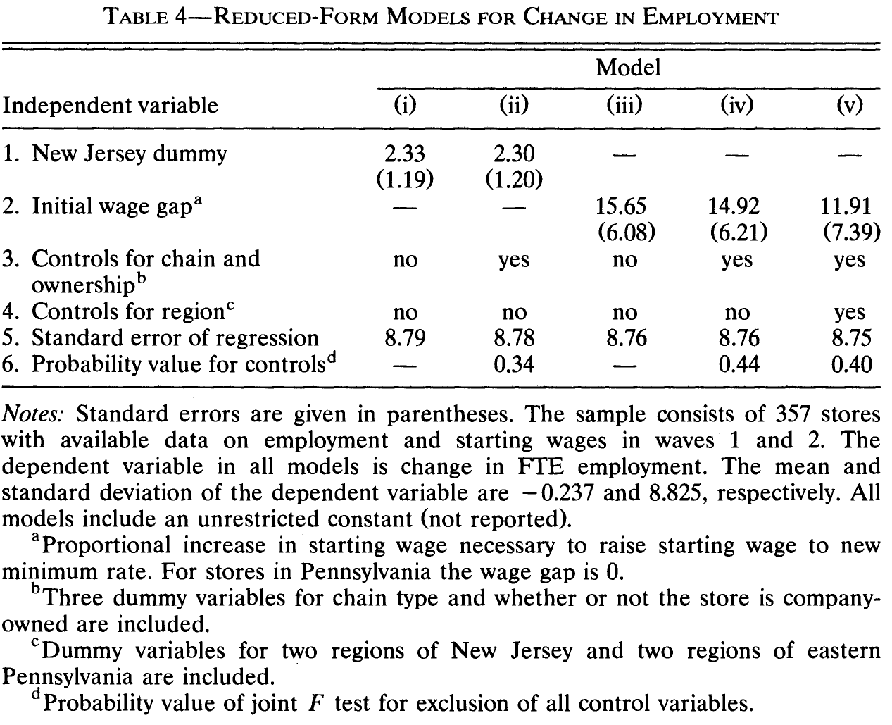
And we can try to replicate those estimates…
# Model (i)/Column 1 (See exercise)

# Model (ii)/Column 2: Controls Chain/Ownership
  fit2 <- lm((y_ft_employment_after-y_ft_employment_before) ~
               d_nj + x_burgerking + x_kfc + x_roys + x_co_owned,
             data = data2)
  summary(fit2)
##
## Call:
## lm(formula = (y_ft_employment_after - y_ft_employment_before) ~
## d_nj + x_burgerking + x_kfc + x_roys + x_co_owned, data = data2)
##
## Residuals:
## Min 1Q Median 3Q Max
## -40.050 -3.685 0.584 4.077 27.169
##
## Coefficients:
## Estimate Std. Error t value Pr(>|t|)
## (Intercept) -2.2067 1.6082 -1.372 0.1709
## d_nj 2.2815 1.1970 1.906 0.0575 .
## x_burgerking 0.7566 1.4911 0.507 0.6122
## x_kfc 0.9912 1.6750 0.592 0.5544
## x_roys -1.3280 1.6811 -0.790 0.4301
## x_co_owned 0.3729 1.0988 0.339 0.7345
## ---
## Signif. codes: 0 '***' 0.001 '**' 0.01 '*' 0.05 '.' 0.1 ' ' 1
##
## Residual standard error: 8.721 on 345 degrees of freedom
## Multiple R-squared: 0.02038, Adjusted R-squared: 0.006185
## F-statistic: 1.436 on 5 and 345 DF, p-value: 0.2108References
Card, David, and Alan B Krueger. 1994. “Minimum Wages and Employment: A Case Study of the Fast-Food Industry in New Jersey and Pennsylvania.” Am. Econ. Rev. 84 (4): 772–93.
Neumark, David, and William Wascher. 2000. “Minimum Wages and Employment: A Case Study of the Fast-Food Industry in New Jersey and Pennsylvania: Comment.” Am. Econ. Rev. 90 (5): 1362–96.
Ropponen, O. 2011. “Reconciling the Evidence of Card and Krueger (1994) and Neumark and Wascher (2000).” J. Appl. Econometrics.