8.10 Lab
8.10.1 Study
- Just as for the exercise on selection-on-observables we’ll use Bauer (2015) again.
- Negative Experiences and Trust: A Causal Analysis of the Effects of Victimization on Generalized Trust (Bauer 2015): What is the causal effect of victimization on social trust?
- Generalized trust is praised by many researchers as the foundation of functioning social systems. An ongoing debate concerns the question whether and to what extent experiences impact individuals’ generalized trust, as measured with the standard trust survey question. So far, reliable empirical evidence regarding the causal effect of experiences on generalized trust is scarce. Studies either do notdirectly measure the quality of experiences or use designs that are prone to selection bias. In the present study, we investigate a unique panel data set from Switzerland that contains measures of trustand measures of negative experiences, i.e. victimization. We use change score analysis and ‘genetic matching’ to investigate the causal effect of victimization on generalized trust and find no substantiallystrong effect that is consistent across panel data waves. (Bauer 2015)
- We use this data because we can discuss several identifcation strategies relying on the same dataset (+ I know it)
8.10.2 Lab: Data
- Data and files can be directly loaded with the command given below or downloaded from the data folder.
data-matching.csv contains a subset of the Bauer (2015) data that we will use for our exercise (Reproduction files). The individual-level dataset covers both victimization (experiencing threats), trust (generalized trust) and various covariates for the period from 2005 to 2008. Below a description where * is replaced with the corresponding year. Analogue to our theoretical sessions treatment variables are generally named d_..., outcome variables y_... and covariates x_.... In this lab session we’ll focus on the variables measured in 2006 (remember that we need to match on pre-treatment values of our covariates), so we could as well take covariate measurements from 2005 with outcome and treatment measured in 2006).
y_trust*: Generalized trust (0-10) at t (Outcome Y)d_threat*: Experiencing a threat (0,1) in year before t (Treatment D)x_age*: Age measure at tx_male*: Gender at t (Male = 1, Female = 0)x_education*: Level of education (0-10) at tx_income*: Income categorical (0,3) at tQ: The data is in wide format. What does that look like?
8.10.3 R Code
We start by importing the data and estimating our standard reg. model in which we control for age, male, income and education. Note that the number of observations equals those in the original dataset.
# Directly import data from shared google folder into R
  data <- readr::read_csv(sprintf("https://docs.google.com/uc?id=%s&export=download", "1WifSODzbCzf0LlP09u9rG914LcUlL08_"))
  # Or download and import: data <- readr::read_csv("data-matching.csv")

fit1 <- lm(y_trust2006 ~ d_threat2006, data = data)
fit2 <- lm(y_trust2006 ~ d_threat2006 + x_age2006 + x_male2006 + x_education2006, data = data)
fit3 <- lm(y_trust2006 ~ d_threat2006 + x_age2006 + x_male2006 + x_education2006 + x_income2006, data = data)
stargazer(fit1, fit2, fit3, type = "html", no.space = TRUE, single.row = TRUE)| Dependent variable: | |||
| y_trust2006 | |||
| (1) | (2) | (3) | |
| d_threat2006 | -0.726*** (0.094) | -0.669*** (0.094) | -0.633*** (0.103) |
| x_age2006 | -0.003* (0.002) | 0.012*** (0.002) | |
| x_male2006 | -0.169*** (0.057) | -0.261*** (0.071) | |
| x_education2006 | 0.134*** (0.010) | 0.133*** (0.012) | |
| x_income2006 | -0.036 (0.035) | ||
| Constant | 6.204*** (0.030) | 5.734*** (0.089) | 5.308*** (0.115) |
| Observations | 6,633 | 6,633 | 4,394 |
| R2 | 0.009 | 0.038 | 0.055 |
| Adjusted R2 | 0.009 | 0.037 | 0.054 |
| Residual Std. Error | 2.293 (df = 6631) | 2.259 (df = 6628) | 2.122 (df = 4388) |
| F Statistic | 60.142*** (df = 1; 6631) | 65.502*** (df = 4; 6628) | 50.706*** (df = 5; 4388) |
| Note: | p<0.1; p<0.05; p<0.01 | ||
8.10.4 Propensity score matching
One of the most popular matching methods was propensity score matching (cf. discussion on the slides). Below an example using our data. We start by importing the data and deleting the missings (row-wise).
# Load the data
data <- readr::read_csv(sprintf("https://docs.google.com/uc?id=%s&export=download", "1WifSODzbCzf0LlP09u9rG914LcUlL08_"))

# Create a new dataset
data2 <- data %>% dplyr::select(y_trust2006, d_threat2006, x_age2006,
                          x_education2006, x_male2006, x_income2006) %>%
                              na.omit() # delete missings
Then we estimate a logistic regression in which the outcome is our treatment variable. In other words we predict whether someone was treated or not using our covariates of interest.
# Estimate the propensity score
# Prob. that someone is victimized as a function of covariates
glm1  <- glm(d_threat2006 ~ x_age2006 + I(x_age2006^2) + x_education2006 +
               I(x_education2006^2) + x_male2006 + x_income2006,
             family=binomial, data=data2)
stargazer(glm1, type = "html")| Dependent variable: | |
| d_threat2006 | |
| x_age2006 | -0.068*** |
| (0.023) | |
| I(x_age20062) | 0.0005* |
| (0.0003) | |
| x_education2006 | -0.019 |
| (0.066) | |
| I(x_education20062) | 0.0004 |
| (0.006) | |
| x_male2006 | 0.452*** |
| (0.108) | |
| x_income2006 | -0.010 |
| (0.060) | |
| Constant | -0.346 |
| (0.371) | |
| Observations | 4,394 |
| Log Likelihood | -1,489.628 |
| Akaike Inf. Crit. | 2,993.256 |
| Note: | p<0.1; p<0.05; p<0.01 |
We use the I() function in the formula because symbols like ^ may have another meaning in a formula than usually (e.g., ^ is used for constructing interactions rather than the expected mathematical power). Here we want to assure that it is understood by R in the mathematical sense (Source).
Subsequently, we use the parameters we estimated in this model (glm1) and predict a propensity score for each individual in our dataset (we can use predict() but we can also access those predictions using glm1$fitted). Conceptually, the propensity score represents the probability that someone receives the treatment as a function of our covariates. We also visualize the propensity score using histograms for treatment (gray) and control (white).
# Calculate (predict) propensity score for each unit and create dataframe
data_treatment_propscore <- data.frame(pr_score = predict(glm1, type = "response"),
                     treatment = glm1$model$d_threat2006)

# Ideally, visualize prop scores by treatment status (histograms)
# Continue using the prop score for matching...
hist(data_treatment_propscore$pr_score[data_treatment_propscore$treatment==0], xlim=c(0,0.5), ylim=c(0,1000),
     main = "Propensity scores and treatment groups", xlab = "Propensity score (gray = treated, white = control)")
hist(data_treatment_propscore$pr_score[data_treatment_propscore$treatment==1], add = TRUE, col = "gray")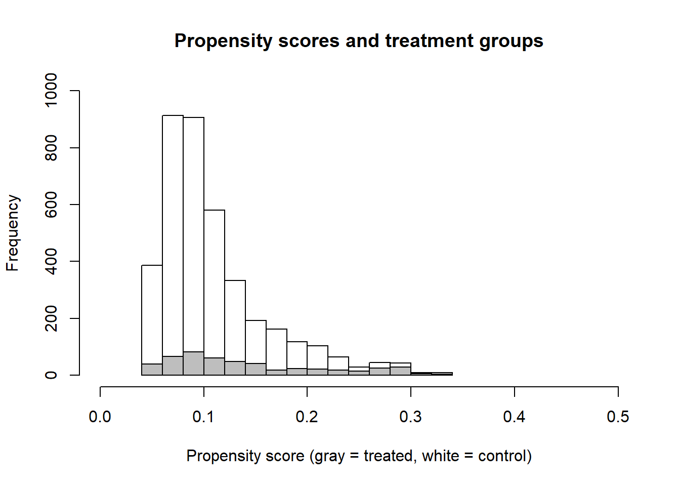
Subsequently, we match not on the covariates themselves but on the individual propensity scores that we predicted before (glm1$fitted is the same as pr_score).
# save data objects
X  <- glm1$fitted
Y  <- data2$y_trust2006
Tr  <- data2$d_threat2006

# Estimating the treatment effect on the treated (the "estimand" option defaults to ATT).
rr  <- Match(Y=Y, Tr=Tr, X=X, M=1)
summary(rr)
##
## Estimate... -0.65135
## AI SE...... 0.12558
## T-stat..... -5.1867
## p.val...... 2.14e-07
##
## Original number of observations.............. 4394
## Original number of treated obs............... 497
## Matched number of observations............... 497
## Matched number of observations (unweighted). 5901Our estimate of the causal effect lies at -0.65 and is statistically significant. As discussed we should check balance (?MatchBalance). The output of MatchBalance is informative but also a bit convoluted (and large) [try running it for yourself].
mb  <- MatchBalance(d_threat2006 ~ x_age2006 + I(x_age2006^2) + x_education2006 +
               I(x_education2006^2) + x_male2006 + x_income2006,
               data=data2, match.out=rr, nboots=10) # use higher nboots in applications
Below we use functions from the cobalt package that allow for a better display of balance (?cobalt).
balance.table <- bal.tab(rr, d_threat2006 ~ x_age2006 + I(x_age2006^2) + x_education2006 +
               I(x_education2006^2) + x_male2006 + x_income2006, data = data2)
balance.table
## Balance Measures
## Type Diff.Adj
## x_age2006 Contin. -0.0194
## I(x_age2006^2) Contin. -0.0250
## x_education2006 Contin. 0.0289
## I(x_education2006^2) Contin. 0.0271
## x_male2006 Binary -0.0103
## x_income2006 Contin. 0.0050
##
## Sample sizes
## Control Treated
## All 3897.000 497
## Matched (ESS) 1190.569 497
## Matched (Unweighted) 2759.000 497
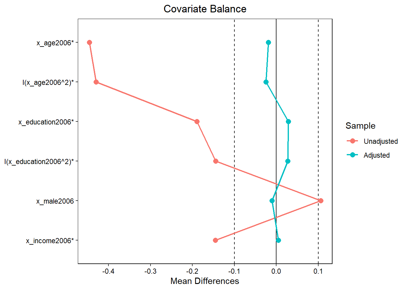
## Unmatched 1138.000 0The love.plot essentially visualizes mean differences (comparing the original dataset and the matched/weighted dataset). It illustrates that covariate mean differences between treatment and control are lower after matching.
8.10.5 Genetic Matching: Single variable
As the name says propensity score matching uses the propensity of getting the treatment (the propensity score) to match treated units to control units. As discussed in class this may induce issues of model dependence. Other methods such as Genetic Matching (Diamond and Sekhon 2013) (see here) match on the covariate values directly.
- “This paper presents genetic matching, a method of multivariate matching that uses an evolutionary search algorithm to determine the weight each covariate is given. Both propensity score matching and matching based on Mahalanobis distance are limiting cases of this method. The algorithm makes transparent certain issues that all matching methods must confront.” (Source)
We start with a simple example in which we match on a single variable x_education2006 (Q: Is that enough in real research?).
# Load the data
data <- readr::read_csv(sprintf("https://docs.google.com/uc?id=%s&export=download", "1WifSODzbCzf0LlP09u9rG914LcUlL08_"))
# Subset the data
data2 <- data %>% dplyr::select(y_trust2006, d_threat2006,
x_education2006)
# then delete missings (Q: Why not the other way round?)
data2 <- na.omit(data2)
# ?GenMatch
# Define covariat matrix, outcome, treatment
X <- as.matrix(data2 %>% dplyr::select(x_education2006))
Y <- data2$y_trust2006 # Define outcome/Response vector
Tr <- data2$d_threat2006 # Define treatment vector
# GenMatch() finds the optimal weight to give each
# covariate in 'X' so as we have achieved balance on the covariates in
# See description http://sekhon.berkeley.edu/papers/MatchingJSS.pdf
gen1 <- GenMatch(Tr = Tr, X = X,
estimand = "ATT",
M = 1,
replace=FALSE,
exact = TRUE,
pop.size=16,
max.generations=10,
wait.generations=1)##
##
## Tue May 12 19:55:19 2020
## Domains:
## 0.000000e+00 <= X1 <= 1.000000e+03
##
## Data Type: Floating Point
## Operators (code number, name, population)
## (1) Cloning........................... 1
## (2) Uniform Mutation.................. 2
## (3) Boundary Mutation................. 2
## (4) Non-Uniform Mutation.............. 2
## (5) Polytope Crossover................ 2
## (6) Simple Crossover.................. 2
## (7) Whole Non-Uniform Mutation........ 2
## (8) Heuristic Crossover............... 2
## (9) Local-Minimum Crossover........... 0
##
## SOFT Maximum Number of Generations: 10
## Maximum Nonchanging Generations: 1
## Population size : 16
## Convergence Tolerance: 1.000000e-03
##
## Not Using the BFGS Derivative Based Optimizer on the Best Individual Each Generation.
## Not Checking Gradients before Stopping.
## Using Out of Bounds Individuals.
##
## Maximization Problem.
## GENERATION: 0 (initializing the population)
## Lexical Fit..... 1.000000e+00 1.000000e+00
## #unique......... 16, #Total UniqueCount: 16
## var 1:
## best............ 1.000000e+00
## mean............ 5.543578e+02
## variance........ 6.037193e+04
##
## GENERATION: 1
## Lexical Fit..... 1.000000e+00 1.000000e+00
## #unique......... 10, #Total UniqueCount: 26
## var 1:
## best............ 1.000000e+00
## mean............ 3.451194e+02
## variance........ 8.664396e+04
##
## GENERATION: 2
## Lexical Fit..... 1.000000e+00 1.000000e+00
## #unique......... 9, #Total UniqueCount: 35
## var 1:
## best............ 1.000000e+00
## mean............ 3.396038e+02
## variance........ 1.087695e+05
##
## 'wait.generations' limit reached.
## No significant improvement in 1 generations.
##
## Solution Lexical Fitness Value:
## 1.000000e+00 1.000000e+00
##
## Parameters at the Solution:
##
## X[ 1] : 1.000000e+00
##
## Solution Found Generation 1
## Number of Generations Run 2
##
## Tue May 12 19:55:26 2020
## Total run time : 0 hours 0 minutes and 7 seconds # with M = 1 each matched unit gets Weight 1, nonmatched ones get 0
#? GenMatch for info, recommendation on pop.size etc.Now that GenMatch() has found the optimal weights, we can estimate our causal effect of interest using those weights:
mgens <- Match(Y=Y, Tr= Tr, X = X,
estimand="ATT",
M = 1,
replace=FALSE,
exact = TRUE,
Weight.matrix = gen1)
summary(mgens)##
## Estimate... -0.74363
## SE......... 0.12921
## T-stat..... -5.7553
## p.val...... 8.6472e-09
##
## Original number of observations.............. 6633
## Original number of treated obs............... 667
## Matched number of observations............... 667
## Matched number of observations (unweighted). 667
##
## Number of obs dropped by 'exact' or 'caliper' 0Q: What do the different elements in the output mean?
Importantly, we have to check whether our matching procedure really produced a matched dataset that is balanced (with exact matching balance should be perfect). We check that below:
##
## ***** (V1) x_education2006 *****
## Before Matching After Matching
## mean treatment........ 4.5892 4.5892
## mean control.......... 5.086 4.5892
## std mean diff......... -15.612 0
##
## mean raw eQQ diff..... 0.49325 0
## med raw eQQ diff..... 0 0
## max raw eQQ diff..... 3 0
##
## mean eCDF diff........ 0.045162 0
## med eCDF diff........ 0.031548 0
## max eCDF diff........ 0.097909 0
##
## var ratio (Tr/Co)..... 1.143 1
## T-test p-value........ 0.00012844 1
## KS Bootstrap p-value.. < 2.22e-16 1
## KS Naive p-value...... 2.0219e-05 1
## KS Statistic.......... 0.097909 0Above we estimated the causal effect and check whether we achieved balance. However, often we want to continue doing analyses based on the matched sample. Below you find the code to extract the matched dataset. Here we can rely on the index vectors index.treated and index.control which contain the observation numbers from the matched observations in the original dataset (Alternatively checkout gen1$matches). We use those vectors to subset the original dataset (and we can also add the vector that includes the weights (if you want to see how the weights change below run GenMatch and Match above with M = 2).
data.matched <- bind_rows(data2 %>% slice(mgens$index.treated), # subset data
data2 %>% slice(mgens$index.control))
data.matched <- bind_cols(data.matched, # Add vector of weights
weights = rep(mgens$weights, 2))Once we obtained the matched dataset we can use it as the basis for a regression model which we do below:
##
## Call:
## lm(formula = y_trust2006 ~ d_threat2006 + x_education2006, data = data.matched)
##
## Residuals:
## Min 1Q Median 3Q Max
## -6.738 -1.153 0.198 1.613 5.059
##
## Coefficients:
## Estimate Std. Error t value Pr(>|t|)
## (Intercept) 5.68499 0.12965 43.850 < 2e-16 ***
## d_threat2006 -0.74363 0.12832 -5.795 8.51e-09 ***
## x_education2006 0.11699 0.02018 5.798 8.38e-09 ***
## ---
## Signif. codes: 0 '***' 0.001 '**' 0.01 '*' 0.05 '.' 0.1 ' ' 1
##
## Residual standard error: 2.343 on 1331 degrees of freedom
## Multiple R-squared: 0.04806, Adjusted R-squared: 0.04663
## F-statistic: 33.6 on 2 and 1331 DF, p-value: 5.813e-15Sometimes we want to compare the matched dataset to the original dataset (or identify units that were not matched). Hence we need to add a dummy variable to the original dataset (that we fed into the matching process) that indicates which observations were used in the matching procedure (we call the data data3 and the dummy matched below):
# Create original dataset with dummy for matching
data3 <- data2
data3$matched <- FALSE
data3$matched[mgens$index.treated] <- TRUE
data3$matched[mgens$index.control] <- TRUENow let’s visually compare the joint distribution of our original dataset and the joint distribution in the matched dataset (we can do that as we have only 3 variables). We can colour the matched observations…
Q: In the legend you can turn on/off to visualized parts of the dataset (unfornately there are only two colors). Which one is the matched and which one the pruned data? Q: There is an observation with the values (Threat = 1, Education = 8, Trust = 0)? What is the control observation for this observation? Is that a case of exact 1 to 1 matching?
8.10.6 Matching on more variables and polynomials..
For illustratory purposes we only matched on one variable above. In applied research we normally match on all relevant covariates (think of the selection on observables assumption!). Below an example..
Important note: Below we also match for the quadratic terms of some of our covariates. At the same time the example code now resorts to exact 1:1 matching without replacement. Since, the covariate values of the matched units in exact matching are exactly the same it does not add any information if we add polynomials of those values (it should also not hurt other than increasing computation time). However, adding polynomials is often done with inexact matching methods as polynomials may reflect other aspects of the covariate distributions (e.g., it’s variance).
data <- readr::read_csv(sprintf("https://docs.google.com/uc?id=%s&export=download", "1WifSODzbCzf0LlP09u9rG914LcUlL08_"))
data2 <- data %>% dplyr::select(y_trust2006, d_threat2006,
x_age2006, x_education2006,
x_male2006, x_income2006)
data2 <- na.omit(data2)
X <- data2 %>% dplyr::select(x_age2006, x_education2006,
x_male2006, x_income2006) # Define covariates
Y <- data2$y_trust2006 # Define outcome/Response vector
Tr <- data2$d_threat2006 # Define treatment vector
# A matrix containing the variables we wish to achieve balance on.
# Default = X
BalanceMat <- cbind(data2$x_age2006, data2$x_education2006,
data2$x_male2006, data2$x_income2006,
I(data2$x_age2006^2), I(data2$x_education2006^2),
I(data2$x_income2006^2))
# GenMatch() finds the optimal weight to give each
# covariate in 'X' so as we have achieved balance on the covariates in
# 'BalanceMat'. Quick example with 'pop.size = 16'
# Should much bigger see
# http://sekhon.berkeley.edu/papers/MatchingJSS.pdf
gen1 <- GenMatch(Tr = Tr, X = X,
BalanceMatrix = BalanceMat,
estimand = "ATT",
M = 1,
replace=FALSE,
exact = TRUE,
pop.size=16,
max.generations=10,
wait.generations=1)##
##
## Tue May 12 19:55:30 2020
## Domains:
## 0.000000e+00 <= X1 <= 1.000000e+03
## 0.000000e+00 <= X2 <= 1.000000e+03
## 0.000000e+00 <= X3 <= 1.000000e+03
## 0.000000e+00 <= X4 <= 1.000000e+03
##
## Data Type: Floating Point
## Operators (code number, name, population)
## (1) Cloning........................... 1
## (2) Uniform Mutation.................. 2
## (3) Boundary Mutation................. 2
## (4) Non-Uniform Mutation.............. 2
## (5) Polytope Crossover................ 2
## (6) Simple Crossover.................. 2
## (7) Whole Non-Uniform Mutation........ 2
## (8) Heuristic Crossover............... 2
## (9) Local-Minimum Crossover........... 0
##
## SOFT Maximum Number of Generations: 10
## Maximum Nonchanging Generations: 1
## Population size : 16
## Convergence Tolerance: 1.000000e-03
##
## Not Using the BFGS Derivative Based Optimizer on the Best Individual Each Generation.
## Not Checking Gradients before Stopping.
## Using Out of Bounds Individuals.
##
## Maximization Problem.
## GENERATION: 0 (initializing the population)
## Lexical Fit..... 1.000000e+00 1.000000e+00 1.000000e+00 1.000000e+00 1.000000e+00 1.000000e+00 1.000000e+00 1.000000e+00 1.000000e+00 1.000000e+00 1.000000e+00 1.000000e+00 1.000000e+00 1.000000e+00
## #unique......... 16, #Total UniqueCount: 16
## var 1:
## best............ 1.000000e+00
## mean............ 4.854027e+02
## variance........ 7.675274e+04
## var 2:
## best............ 1.000000e+00
## mean............ 5.408518e+02
## variance........ 6.340809e+04
## var 3:
## best............ 1.000000e+00
## mean............ 4.955960e+02
## variance........ 9.396228e+04
## var 4:
## best............ 1.000000e+00
## mean............ 4.505653e+02
## variance........ 7.423558e+04
##
## GENERATION: 1
## Lexical Fit..... 1.000000e+00 1.000000e+00 1.000000e+00 1.000000e+00 1.000000e+00 1.000000e+00 1.000000e+00 1.000000e+00 1.000000e+00 1.000000e+00 1.000000e+00 1.000000e+00 1.000000e+00 1.000000e+00
## #unique......... 10, #Total UniqueCount: 26
## var 1:
## best............ 1.000000e+00
## mean............ 3.491538e+02
## variance........ 5.991935e+04
## var 2:
## best............ 1.000000e+00
## mean............ 4.051341e+02
## variance........ 1.277078e+05
## var 3:
## best............ 1.000000e+00
## mean............ 4.541212e+02
## variance........ 8.986205e+04
## var 4:
## best............ 1.000000e+00
## mean............ 5.637786e+02
## variance........ 1.318397e+05
##
## GENERATION: 2
## Lexical Fit..... 1.000000e+00 1.000000e+00 1.000000e+00 1.000000e+00 1.000000e+00 1.000000e+00 1.000000e+00 1.000000e+00 1.000000e+00 1.000000e+00 1.000000e+00 1.000000e+00 1.000000e+00 1.000000e+00
## #unique......... 8, #Total UniqueCount: 34
## var 1:
## best............ 1.000000e+00
## mean............ 2.691684e+02
## variance........ 4.410993e+04
## var 2:
## best............ 1.000000e+00
## mean............ 4.014683e+02
## variance........ 1.703935e+05
## var 3:
## best............ 1.000000e+00
## mean............ 3.778131e+02
## variance........ 1.038113e+05
## var 4:
## best............ 1.000000e+00
## mean............ 5.364358e+02
## variance........ 1.593737e+05
##
## 'wait.generations' limit reached.
## No significant improvement in 1 generations.
##
## Solution Lexical Fitness Value:
## 1.000000e+00 1.000000e+00 1.000000e+00 1.000000e+00 1.000000e+00 1.000000e+00 1.000000e+00 1.000000e+00 1.000000e+00 1.000000e+00 1.000000e+00 1.000000e+00 1.000000e+00 1.000000e+00
##
## Parameters at the Solution:
##
## X[ 1] : 1.000000e+00
## X[ 2] : 1.000000e+00
## X[ 3] : 1.000000e+00
## X[ 4] : 1.000000e+00
##
## Solution Found Generation 1
## Number of Generations Run 2
##
## Tue May 12 19:55:32 2020
## Total run time : 0 hours 0 minutes and 2 secondsNow that GenMatch() has found the optimal weights, let’s estimate our causal effect of interest using those weights:
mgens <- Match(Y=Y, Tr= Tr, X = X,
estimand = "ATT",
M = 1,
replace=FALSE,
exact = TRUE,
Weight.matrix = gen1)
summary(mgens)##
## Estimate... -0.6738
## SE......... 0.15485
## T-stat..... -4.3512
## p.val...... 1.3541e-05
##
## Original number of observations.............. 4394
## Original number of treated obs............... 497
## Matched number of observations............... 374
## Matched number of observations (unweighted). 374
##
## Number of obs dropped by 'exact' or 'caliper' 123And just as before we check the balance:
#Let's determine if balance has actually been obtained on the variables of interest
mb <- MatchBalance(Tr ~ x_age2006 + x_education2006 +
x_male2006 + x_income2006 +
I(x_age2006^2) + I(x_education2006^2) +
I(x_income2006^2),
match.out = mgens, nboots = 10, data = data2) ##
## ***** (V1) x_age2006 *****
## Before Matching After Matching
## mean treatment........ 35.714 34.516
## mean control.......... 42.054 34.516
## std mean diff......... -44.504 0
##
## mean raw eQQ diff..... 6.3581 0
## med raw eQQ diff..... 6 0
## max raw eQQ diff..... 12 0
##
## mean eCDF diff........ 0.090769 0
## med eCDF diff........ 0.090635 0
## max eCDF diff........ 0.20444 0
##
## var ratio (Tr/Co)..... 1.113 1
## T-test p-value........ < 2.22e-16 1
## KS Bootstrap p-value.. < 2.22e-16 1
## KS Naive p-value...... 2.2204e-16 1
## KS Statistic.......... 0.20444 0
##
##
## ***** (V2) x_education2006 *****
## Before Matching After Matching
## mean treatment........ 4.9577 4.6631
## mean control.......... 5.5486 4.6631
## std mean diff......... -18.931 0
##
## mean raw eQQ diff..... 0.58551 0
## med raw eQQ diff..... 0 0
## max raw eQQ diff..... 3 0
##
## mean eCDF diff........ 0.053716 0
## med eCDF diff........ 0.047811 0
## max eCDF diff........ 0.10036 0
##
## var ratio (Tr/Co)..... 1.1602 1
## T-test p-value........ 6.9401e-05 1
## KS Bootstrap p-value.. < 2.22e-16 1
## KS Naive p-value...... 0.00027872 1
## KS Statistic.......... 0.10036 0
##
##
## ***** (V3) x_male2006 *****
## Before Matching After Matching
## mean treatment........ 0.5835 0.58556
## mean control.......... 0.47806 0.58556
## std mean diff......... 21.367 0
##
## mean raw eQQ diff..... 0.10463 0
## med raw eQQ diff..... 0 0
## max raw eQQ diff..... 1 0
##
## mean eCDF diff........ 0.05272 0
## med eCDF diff........ 0.05272 0
## max eCDF diff........ 0.10544 0
##
## var ratio (Tr/Co)..... 0.9757 1
## T-test p-value........ 8.8711e-06 1
##
##
## ***** (V4) x_income2006 *****
## Before Matching After Matching
## mean treatment........ 1.2636 1.2594
## mean control.......... 1.4285 1.2594
## std mean diff......... -14.494 0
##
## mean raw eQQ diff..... 0.16298 0
## med raw eQQ diff..... 0 0
## max raw eQQ diff..... 1 0
##
## mean eCDF diff........ 0.041238 0
## med eCDF diff........ 0.050727 0
## max eCDF diff........ 0.063499 0
##
## var ratio (Tr/Co)..... 0.99178 1
## T-test p-value........ 0.0024519 1
## KS Bootstrap p-value.. < 2.22e-16 1
## KS Naive p-value...... 0.057186 1
## KS Statistic.......... 0.063499 0
##
##
## ***** (V5) I(x_age2006^2) *****
## Before Matching After Matching
## mean treatment........ 1478 1376.1
## mean control.......... 1950.8 1376.1
## std mean diff......... -42.916 0
##
## mean raw eQQ diff..... 477.63 0
## med raw eQQ diff..... 520 0
## max raw eQQ diff..... 1680 0
##
## mean eCDF diff........ 0.090769 0
## med eCDF diff........ 0.090635 0
## max eCDF diff........ 0.20444 0
##
## var ratio (Tr/Co)..... 0.93602 1
## T-test p-value........ < 2.22e-16 1
## KS Bootstrap p-value.. < 2.22e-16 1
## KS Naive p-value...... 2.2204e-16 1
## KS Statistic.......... 0.20444 0
##
##
## ***** (V6) I(x_education2006^2) *****
## Before Matching After Matching
## mean treatment........ 34.302 31.529
## mean control.......... 39.182 31.529
## std mean diff......... -14.429 0
##
## mean raw eQQ diff..... 4.8551 0
## med raw eQQ diff..... 0 0
## max raw eQQ diff..... 32 0
##
## mean eCDF diff........ 0.053716 0
## med eCDF diff........ 0.047811 0
## max eCDF diff........ 0.10036 0
##
## var ratio (Tr/Co)..... 0.99376 1
## T-test p-value........ 0.0025592 1
## KS Bootstrap p-value.. < 2.22e-16 1
## KS Naive p-value...... 0.00027872 1
## KS Statistic.......... 0.10036 0
##
##
## ***** (V7) I(x_income2006^2) *****
## Before Matching After Matching
## mean treatment........ 2.8893 2.9759
## mean control.......... 3.3464 2.9759
## std mean diff......... -13.196 0
##
## mean raw eQQ diff..... 0.45272 0
## med raw eQQ diff..... 0 0
## max raw eQQ diff..... 5 0
##
## mean eCDF diff........ 0.041238 0
## med eCDF diff........ 0.050727 0
## max eCDF diff........ 0.063499 0
##
## var ratio (Tr/Co)..... 0.927 1
## T-test p-value........ 0.0059771 1
## KS Bootstrap p-value.. < 2.22e-16 1
## KS Naive p-value...... 0.057186 1
## KS Statistic.......... 0.063499 0
##
##
## Before Matching Minimum p.value: < 2.22e-16
## Variable Name(s): x_age2006 x_education2006 x_income2006 I(x_age2006^2) I(x_education2006^2) I(x_income2006^2) Number(s): 1 2 4 5 6 7
##
## After Matching Minimum p.value: 1Or even better we visualize it:
# Visualize balance with bal.tab (cobalt package)
balance.table <- bal.tab(mgens, d_threat2006 ~ x_age2006 + x_education2006 +
x_male2006 + x_income2006 +
I(x_age2006^2) + I(x_education2006^2) +
I(x_income2006^2), data = data2)
love.plot(balance.table,
          threshold =.1,
          line = TRUE,
stars = "std") # check ?love.plot; * variables have been standardized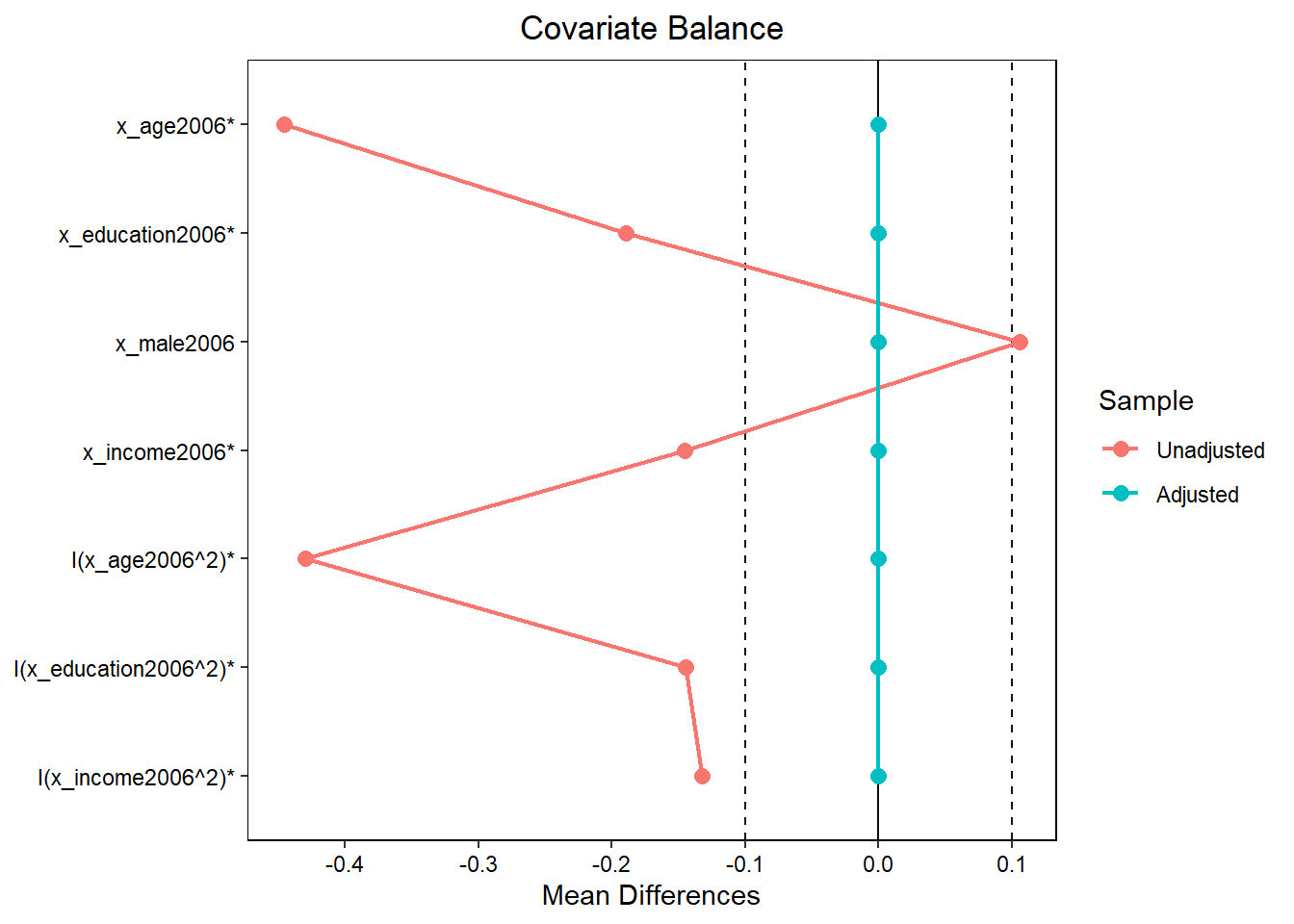
References
Bauer, Paul C. 2015. “Negative Experiences and Trust: A Causal Analysis of the Effects of Victimization on Generalized Trust.” Eur. Sociol. Rev. 31 (4): 397–417.
Diamond, Alexis, and Jasjeet S Sekhon. 2013. “Genetic Matching for Estimating Causal Effects: A General Multivariate Matching Method for Achieving Balance in Observational Studies.” The Review of Economics and Statistics 95 (3): 932–45.