13.11 Lab: R Code
13.11.1 Run the following functions
13.11.2 Load data & install packages
  # set.seed(48104) # ?set.seed

# Load data
  data_rdd <- foreign::read.dta("https://docs.google.com/uc?id=1xWHmST5FYcfLxe9V7Hwqd2LIy_A3ninG&export=download")
  # data_rdd <- foreign::read.dta("www/rdd-fouirnaies_hall_financial_incumbency_advantage.dta")
  data_rdd <- data_rdd %>% rename(x_score_victorymargin = rv,
                                  y_donationshare = dv_money,
                                  cov_statelevel = statelevel,
                                  cov_total_race_money = total_race_money,
                                  cov_total_votes = total_votes,
                                  cov_dem_inc = dem_inc,
                                  cov_rep_inc = rep_inc,
                                  cov_total_group_money = total_group_money) %>%
    dplyr::select(x_score_victorymargin,
           y_donationshare,
           cov_statelevel,
           cov_total_race_money,
           cov_total_votes,
           cov_dem_inc,
           cov_rep_inc,
           cov_total_group_money,
           state,
           dist,
           year)
13.11.3 Explore data and subsetting
# names(data_rdd) # Show variables
# View(data_rdd)

# Filter out state legislative district level
table(data_rdd$cov_statelevel) # How many state-level elections are there?| 0 | 1 |
|---|---|
| 6533 | 32670 |
13.11.4 Summary statistics + graphs
Below we inspect the variables.
Q: What the min. and max. values of the variable x_score_victorymargin mean substantively? And the same for y_donationshare?
# Summarize score variable (also called running variable): Vote share
summary(data_rdd$x_score_victorymargin)| Min. | 1st Qu. | Median | Mean | 3rd Qu. | Max. |
|---|---|---|---|---|---|
| -50 | -16.05517 | 0.134985 | 1.357636 | 20.07864 | 50 |
| Min. | 1st Qu. | Median | Mean | 3rd Qu. | Max. | NA’s |
|---|---|---|---|---|---|---|
| 0 | 6.540446 | 50.60789 | 50.78094 | 96.80258 | 100 | 5467 |
  # Share of donations flowing to the incumbent’s party

# Plot oucome var vs. score variable
p = qplot(x_score_victorymargin, y_donationshare, data=data_rdd) +
  xlab("Democratic margin of victory at t") +
  ylab("Democratic share of contributions at t+1")
p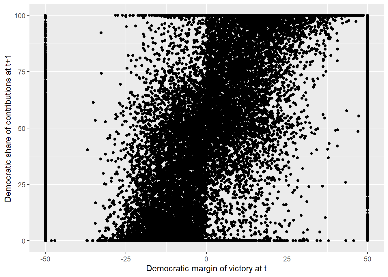
We can do the same with plotly..
data_rdd$colour[data_rdd$x_score_victorymargin<=0] <- "Treated"
data_rdd$colour[data_rdd$x_score_victorymargin>0] <- "Control"

plot_ly(data = data_rdd,
        type = "scatter",
        mode = "markers",
        x = data_rdd$x_score_victorymargin,
        y = data_rdd$y_donationshare,
        color = data_rdd$colour,
        marker = list(size=3)) %>%
    layout(xaxis = list(title = "Democratic margin of victory at t", dtick = 25),
                yaxis = list(title = "Democratic share of contributions at t+1"))
13.11.5 Continuity-based analysis
13.11.5.1 Density test
First, we can check the density of the running/score variable as a falsification test. If the density (the number of observations) below cutoff is considerably different from the one above it would indicate that individuals/politicians/parties in districts have the possibility to manipulate their scores.
Q: What would you say? Does it look as if the density is discontinuous at the cutoff?
##
## RD Manipulation Test using local polynomial density estimation.
##
## Number of obs =       32670
## Model =               unrestricted
## Kernel =              triangular
## BW method =           comb
## VCE method =          jackknife
##
## Cutoff c = 0          Left of c           Right of c
## Number of obs         16281               16389
## Eff. Number of obs    2770                3176
## Order est. (p)        2                   2
## Order bias (q)        3                   3
## BW est. (h)           5.458               6.935
##
## Method                T                   P > |T|
## Robust                -0.9165             0.3594
# histogram of density test
p = ggplot(data_rdd,aes(x=x_score_victorymargin, fill = factor(data_rdd$x_score_victorymargin>0)))+geom_histogram(binwidth=0.5)+xlim(-25,25)+geom_vline(xintercept = 0)+xlab("Democratic vote share at t")+scale_colour_manual(values = c("red","blue"))+theme_bw()+theme(legend.position='none')
p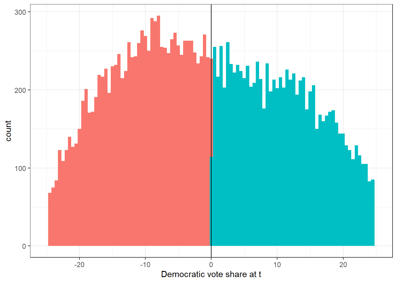
13.11.5.2 Covariates as outcomes
Next, Skovron and Titiunik (2015, 30) investigate the effect of the treatment on five predetermined covariates (see Table 1 below) but find no treatment effect for any of them. N“ear the cutoff, treated units are similar to control units. The idea is simply that, if units lack the ability to precisely manipulate the value of the score they receive, units just above and just below the cutoff should be similar in all those characteristics that could not have been affected by the treatment” (Skovron and Titiunik 2015, 28).
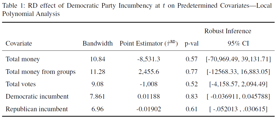
Skovron & Titiunik 2015, Tab. 1, p.31
We can reproduce and graph these results (for Total money and Total money from groups) using the code below.
# Total money in race
  summary(rdrobust(data_rdd$cov_total_race_money, data_rdd$x_score_victorymargin, all=TRUE))
## [1] "Mass points detected in the running variable."
## Call: rdrobust
##
## Number of Obs. 32670
## BW type mserd
## Kernel Triangular
## VCE method NN
##
## Number of Obs. 16281 16389
## Eff. Number of Obs. 5798 4920
## Order est. (p) 1 1
## Order bias (q) 2 2
## BW est. (h) 11.114 11.114
## BW bias (b) 17.304 17.304
## rho (h/b) 0.642 0.642
## Unique Obs. 11187 10946
##
## =============================================================================
## Method Coef. Std. Err. z P>|z| [ 95% C.I. ]
## =============================================================================
## Conventional -7945.069 23075.255 -0.344 0.731[-53171.737 , 37281.599]
## Bias-Corrected-14849.630 23075.255 -0.644 0.520[-60076.298 , 30377.038]
## Robust-14849.630 27623.054 -0.538 0.591[-68989.820 , 39290.561]
## ============================================================================= rdplot(data_rdd$cov_total_race_money,data_rdd$x_score_victorymargin,
x.lim = c(-10,10),
y.lim = c(0,400000),
x.lab="Democratic margin of victory at t",
y.lab="Total money in race at t+1", title = "")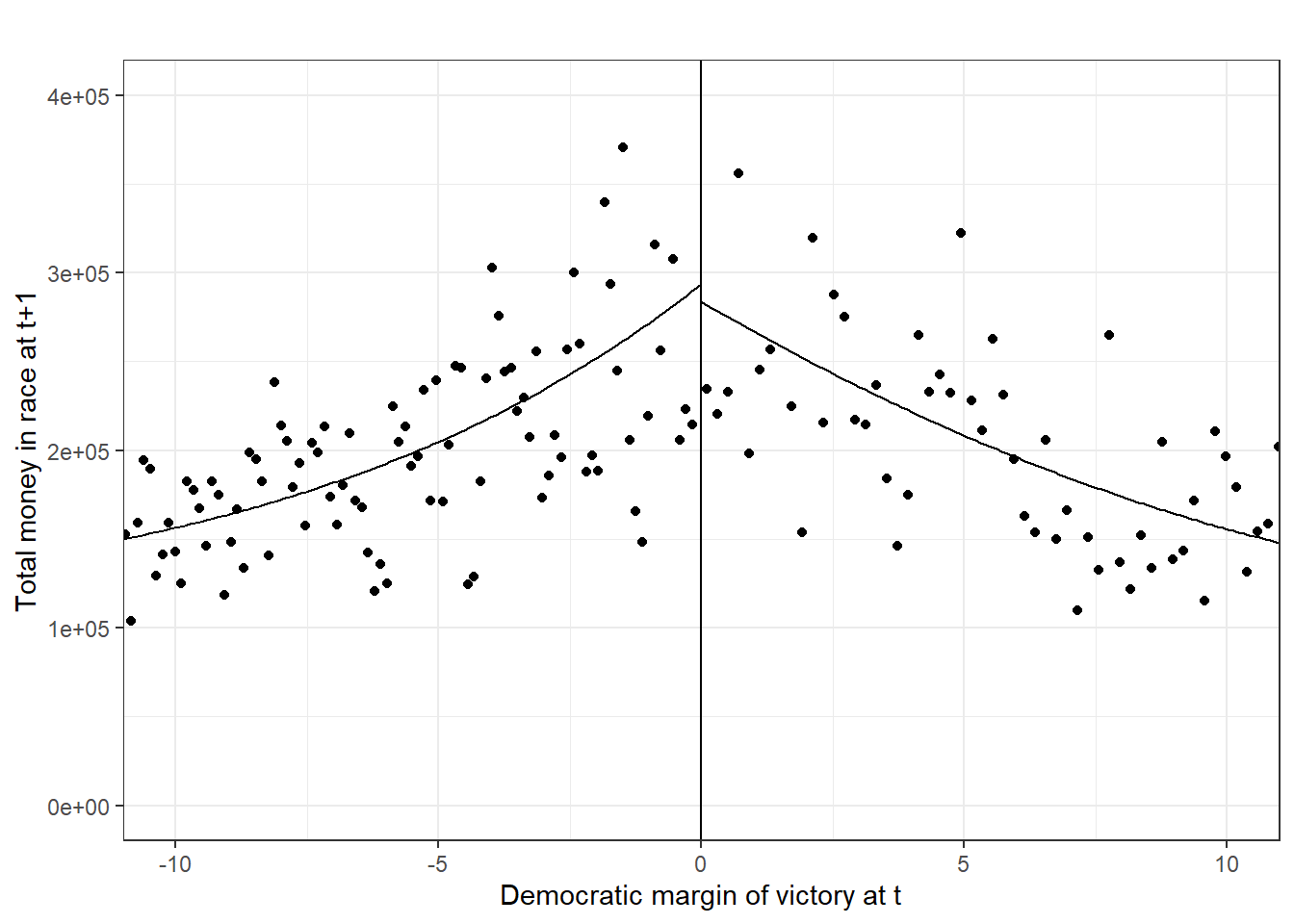
# Total votes in race
  summary(rdrobust(data_rdd$cov_total_votes,data_rdd$x_score_victorymargin,all=TRUE))
## [1] "Mass points detected in the running variable."
## Call: rdrobust
##
## Number of Obs. 32670
## BW type mserd
## Kernel Triangular
## VCE method NN
##
## Number of Obs. 16281 16389
## Eff. Number of Obs. 3077 2781
## Order est. (p) 1 1
## Order bias (q) 2 2
## BW est. (h) 6.024 6.024
## BW bias (b) 10.430 10.430
## rho (h/b) 0.578 0.578
## Unique Obs. 11187 10946
##
## =============================================================================
## Method Coef. Std. Err. z P>|z| [ 95% C.I. ]
## =============================================================================
## Conventional -1629.150 1655.583 -0.984 0.325 [-4874.033 , 1615.732]
## Bias-Corrected -2160.740 1655.583 -1.305 0.192 [-5405.623 , 1084.143]
## Robust -2160.740 1921.312 -1.125 0.261 [-5926.442 , 1604.962]
## ============================================================================= rdplot(data_rdd$cov_total_votes,data_rdd$x_score_victorymargin,
x.lim = c(-10,10),
y.lim = c(0,50000),
x.lab="Democratic margin of victory at t",
y.lab="Total votes in race at t+1", title = "")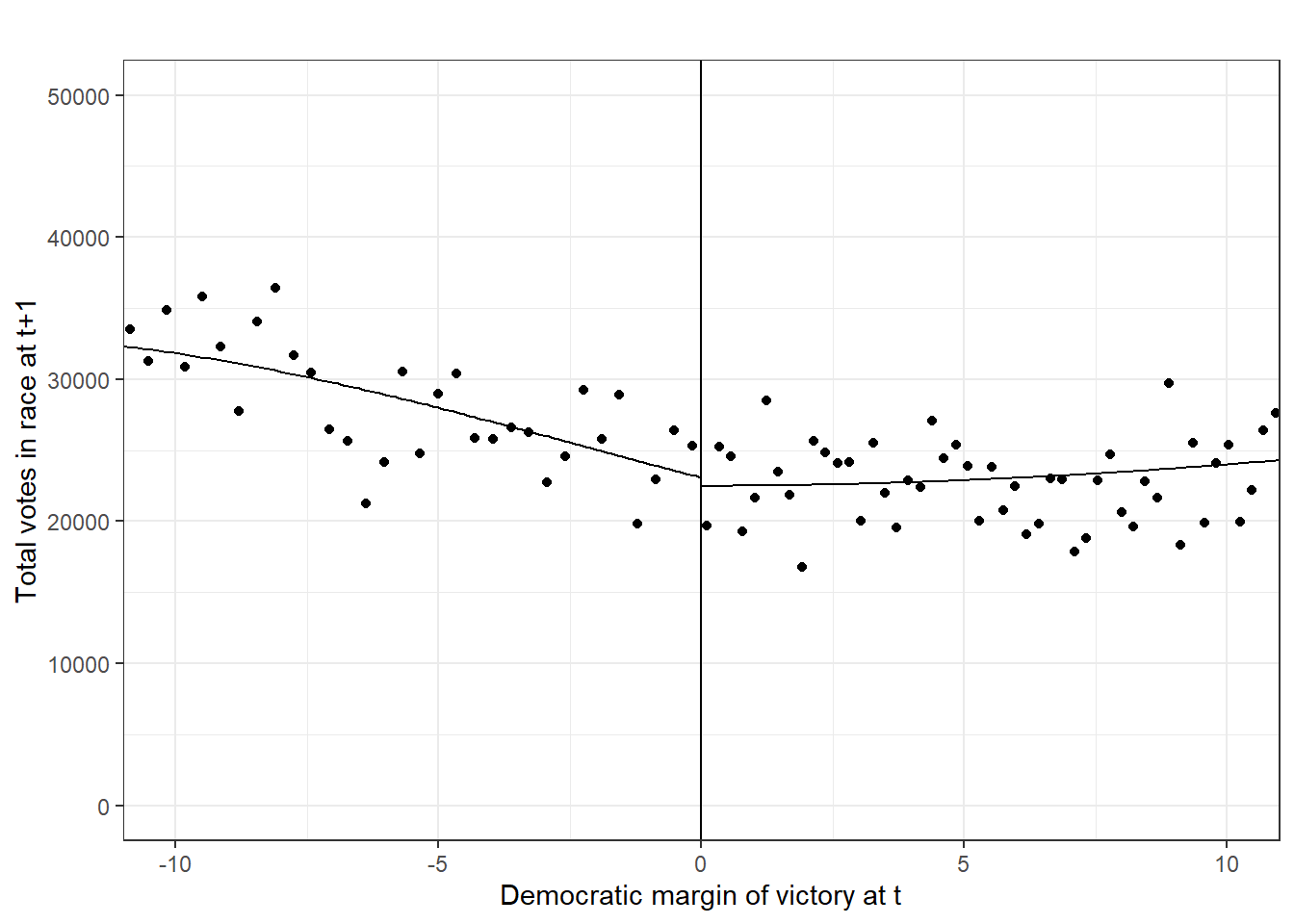
13.11.5.3 Estimation of RD effect
Below we finally estimate the RD effect. Table 2 displays the estimates.
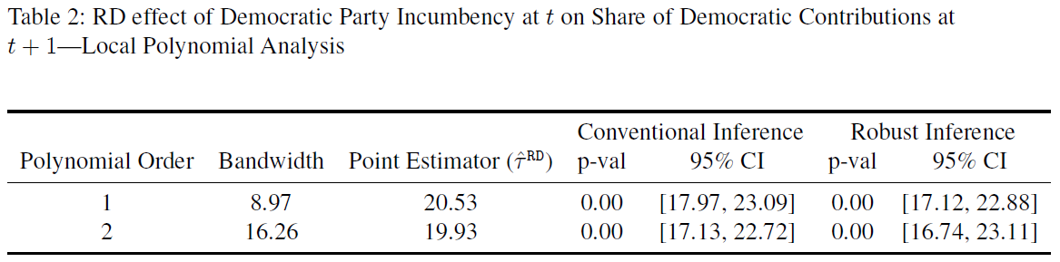
Skovron & Titiunik 2015, Tab. 1, p.31
We can reproduce this as follows relying on the rdrobust function (See ?rdrobust).
Before we can fit the local polynomial functions we have to choose a bandwidth, i.e. the width or region of the neighborhood around the cutoff for which we accept the data. This choice involves a bias-variance trade-off. A large bandwidth may result in in a large bias if the unknown function differs considerably from the polynomial approximation. At the same time it will decrease the variance of the estimated coefficients because we have more observations (and the other way round).
The rdrobust function chooses optimal bandwidth and produces robust bias-corrected confidence intervals (read more on this in Skovron and Titiunik (2015) and related publications, ?rdrobust).
  #?rdrobust
  set.seed(48104)
# RD Effect for main outcome variable
  # ==> Local linear polynomial estimation with optimal bandwidth
  fit <- rdrobust(data_rdd$y_donationshare, data_rdd$x_score_victorymargin, c = 0, all=TRUE)
## [1] "Mass points detected in the running variable."## Call: rdrobust
##
## Number of Obs. 27203
## BW type mserd
## Kernel Triangular
## VCE method NN
##
## Number of Obs. 13292 13911
## Eff. Number of Obs. 3994 3435
## Order est. (p) 1 1
## Order bias (q) 2 2
## BW est. (h) 9.270 9.270
## BW bias (b) 19.028 19.028
## rho (h/b) 0.487 0.487
## Unique Obs. 9006 9199
##
## =============================================================================
## Method Coef. Std. Err. z P>|z| [ 95% C.I. ]
## =============================================================================
## Conventional 20.532 1.285 15.984 0.000 [18.014 , 23.049]
## Bias-Corrected 19.971 1.285 15.547 0.000 [17.453 , 22.489]
## Robust 19.971 1.423 14.038 0.000 [17.183 , 22.760]
## =============================================================================
You can also chose particular bandwidths specifying the h argument. Fouirnaies/Hall use bandwidths of 1, 2, and 3 percentage points… (below just 1 but try playing around with the values)
## [1] "Mass points detected in the running variable."
## Call: rdrobust
##
## Number of Obs.                27203
## BW type                      Manual
## Kernel                   Triangular
## VCE method                       NN
##
## Number of Obs.               13292       13911
## Eff. Number of Obs.            415         400
## Order est. (p)                   1           1
## Order bias  (q)                  2           2
## BW est. (h)                  1.000       1.000
## BW bias (b)                  1.000       1.000
## rho (h/b)                    1.000       1.000
## Unique Obs.                   9006        9199
##
## =============================================================================
##         Method     Coef. Std. Err.         z     P>|z|      [ 95% C.I. ]
## =============================================================================
##   Conventional    23.642     3.830     6.173     0.000    [16.136 , 31.148]
## Bias-Corrected    23.604     3.830     6.164     0.000    [16.098 , 31.110]
##         Robust    23.604     5.520     4.276     0.000    [12.785 , 34.424]
## =============================================================================
And we can plot the results. CCT bandwidth in main estimation was about 9 (see above) so we restrict the x axis to (-10,10).
rdplot(data_rdd$y_donationshare,data_rdd$x_score_victorymargin,x.lim=c(-10,10),
       y.lab="Democratic share of contributions at t+1", title = "RDD Estimate")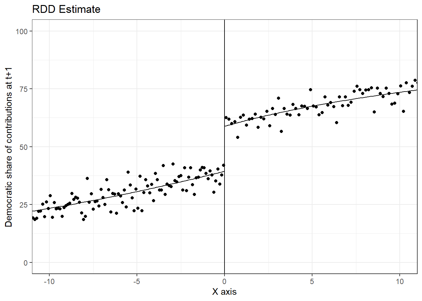
Naturally, focusing on that subset on the x-Axis does not give us the whole picture. Hence, we a a graph that visualizes the whole data range. Q: What do you see here?
# RD plot using whole data range
  rdplot(data_rdd$y_donationshare,data_rdd$x_score_victorymargin,
         x.lab="Democratic margin of victory at t",
         y.lab="Democratic share of contributions at t+1",
         title = "RDD Estimate")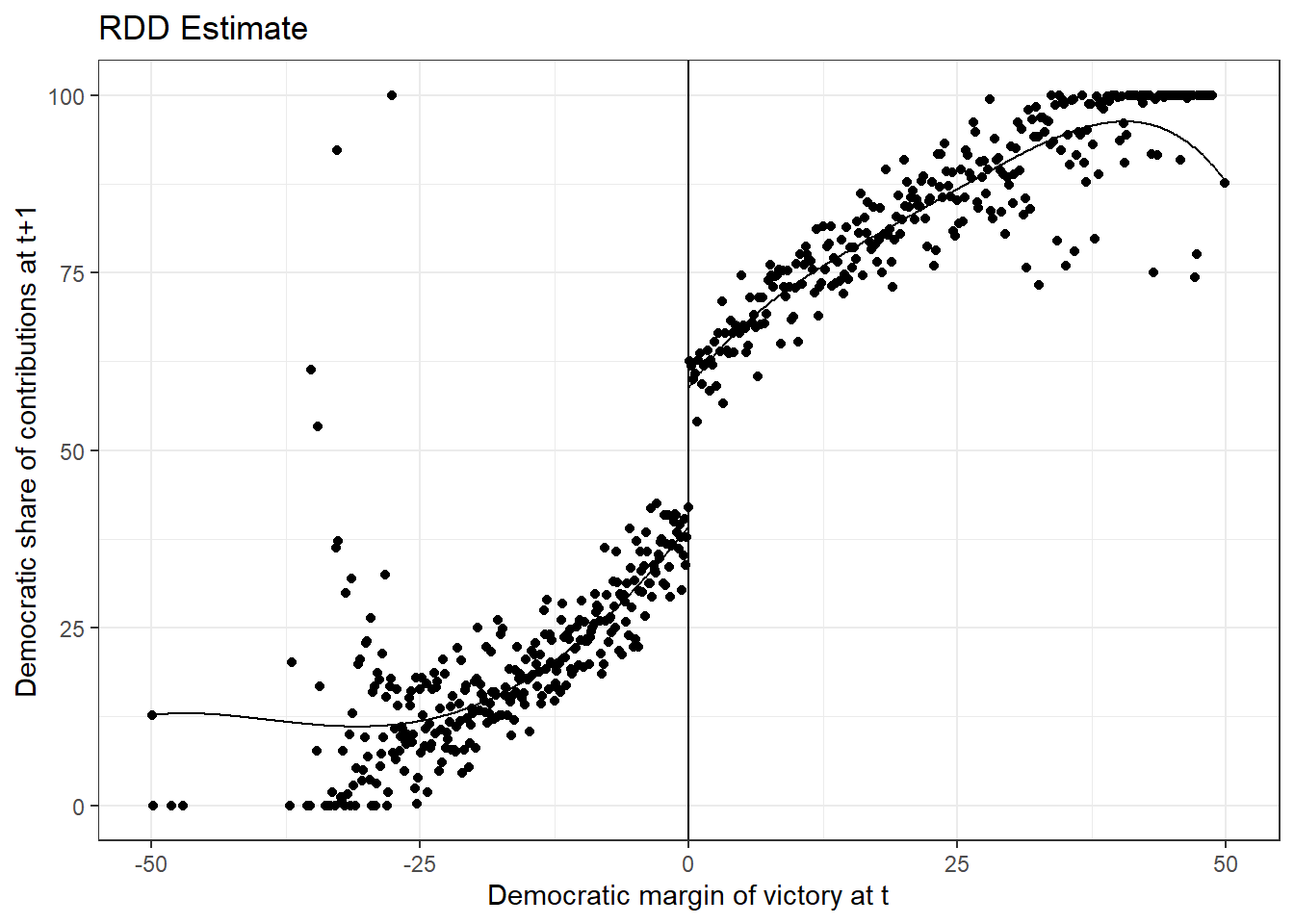
Finally, we have the possibility to test (and should) whether we can find treatment effects for placebo cutoffs. There shouldn’t be any.
# cutoff c = 1
summary(rdrobust(data_rdd$y_donationshare,data_rdd$x_score_victorymargin, c = 1 ,all=TRUE))
## [1] "Mass points detected in the running variable."
## Call: rdrobust
##
## Number of Obs. 27203
## BW type mserd
## Kernel Triangular
## VCE method NN
##
## Number of Obs. 13692 13511
## Eff. Number of Obs. 1271 1204
## Order est. (p) 1 1
## Order bias (q) 2 2
## BW est. (h) 3.125 3.125
## BW bias (b) 8.042 8.042
## rho (h/b) 0.389 0.389
## Unique Obs. 9406 8799
##
## =============================================================================
## Method Coef. Std. Err. z P>|z| [ 95% C.I. ]
## =============================================================================
## Conventional -1.994 2.257 -0.883 0.377 [-6.418 , 2.430]
## Bias-Corrected -3.071 2.257 -1.361 0.174 [-7.495 , 1.352]
## Robust -3.071 2.394 -1.283 0.200 [-7.764 , 1.621]
## =============================================================================# cutoff c = -3
summary(rdrobust(data_rdd$y_donationshare,data_rdd$x_score_victorymargin, c = -3 ,all=TRUE))## [1] "Mass points detected in the running variable."
## Call: rdrobust
##
## Number of Obs. 27203
## BW type mserd
## Kernel Triangular
## VCE method NN
##
## Number of Obs. 12055 15148
## Eff. Number of Obs. 2005 1906
## Order est. (p) 1 1
## Order bias (q) 2 2
## BW est. (h) 4.668 4.668
## BW bias (b) 9.363 9.363
## rho (h/b) 0.499 0.499
## Unique Obs. 7769 10436
##
## =============================================================================
## Method Coef. Std. Err. z P>|z| [ 95% C.I. ]
## =============================================================================
## Conventional -2.139 1.801 -1.188 0.235 [-5.670 , 1.391]
## Bias-Corrected -2.930 1.801 -1.626 0.104 [-6.460 , 0.601]
## Robust -2.930 1.997 -1.467 0.142 [-6.844 , 0.984]
## =============================================================================References
Skovron, Christopher, and Rocıo Titiunik. 2015. “A Practical Guide to Regression Discontinuity Designs in Political Science.”