26.1 g200 hadron
first we read the header
to.read = file("../g200/G2t_T64_L20_msq0-1.200000_msq1-0.550000_l00.000000_l10.000000_mu0.000000_g200.000000_rep0_bin1000_merged_bin100", "rb")
if(!exists("foo", mode="function")) source("read_header.R")
header<-read_header(to.read)
## Warning in readChar(to.read, nchars = 100, useBytes = 100): truncating string
## with embedded nuls#header26.1.1 Reading the configuration
We read the configuration from the file in to the three dimensional array d[correlator, time, configuration]
configurations <- list()
d<-array(dim = c(header$ncorr, header$L[1], header$confs) )

for (iconf in  c(1:header$confs)){
  configurations<-append(configurations, readBin(to.read, integer(),n = 1, endian = "little"))
  for(t in c(1:header$L[1] ) ){
    for (corr in  c(1:header$ncorr)){
          d[corr, t, iconf]<-readBin(to.read, double(),n = 1, endian = "little")
      }
  }
}
26.1.2 GEVP
first we define the correlator number that correspond to the correlator we want in the GEVP
###########
n_00<-0+1   # <phi0   phi0  >
n_01<-129+1 # <phi0^3   phi0  >
n_02<-127+1 # <phi0   phi1  >


n_11<-5+1   # <phi0^3   phi0^3  >
n_12<-128+1 # <phi0^3   phi1  >


n_22<-1+1   # <phi1   phi1  >
#######
n_03<-188+1 # <phi0     phi0^2phi1  >
n_13<-189+1 # <phi0^3   phi0^2phi1  >
n_23<-190+1 # <phi1^3   phi0^2phi1  >
n_33<-187+1 # <phi0^2phi1   phi0^2phi1  >
with the above correlator we build the GEVP between the operators \(\phi_1\) and \(\phi_0^3\)
mycf<- cf()
# for (n in c(n_00,n_01,n_02,
#             n_01,n_11,n_12,
#             n_02,n_12,n_22)){

for (n in c(
            n_11,n_12,
            n_12,n_22)){

  cf_tmp <- cf_meta(nrObs =1, Time = header$L[1], nrStypes = 1)
  cf_tmp <- cf_orig(cf_tmp, cf = t(d[n, ,]))
  cf_tmp <- symmetrise.cf(cf_tmp, sym.vec = c(1))
  mycf<- c(mycf, cf_tmp)

}
# Bootstrap cf
boot.R <- 150
boot.l <- 1
seed <- 1433567
cfb <- bootstrap.cf(cf=mycf, boot.R=boot.R, boot.l=boot.l, seed=seed)
26.1.3 Effective mass
cor1 <- extractSingleCor.cf(cf=cfb, id=1)
cor1.effmass <- bootstrap.effectivemass(cf=cor1)
cor2_g200 <- extractSingleCor.cf(cf=cfb, id=2)
cor2.effmass <- bootstrap.effectivemass(cf=cor2_g200)
cor3 <- extractSingleCor.cf(cf=cfb, id=4)
cor3.effmass <- bootstrap.effectivemass(cf=cor3)
plot(cor1.effmass, ylab="a Meff", xlab="t/a", xlim=c(0,20),ylim=c(0.3,0.8))
plot(cor2.effmass, rep=TRUE, col="red")
plot(cor3.effmass, rep=TRUE, col="blue")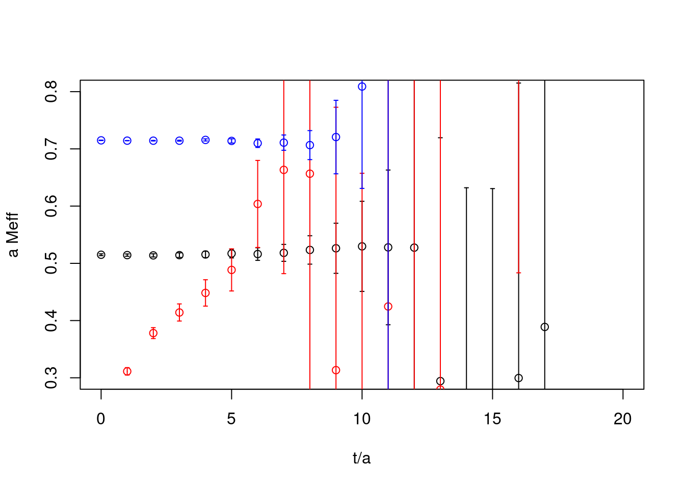
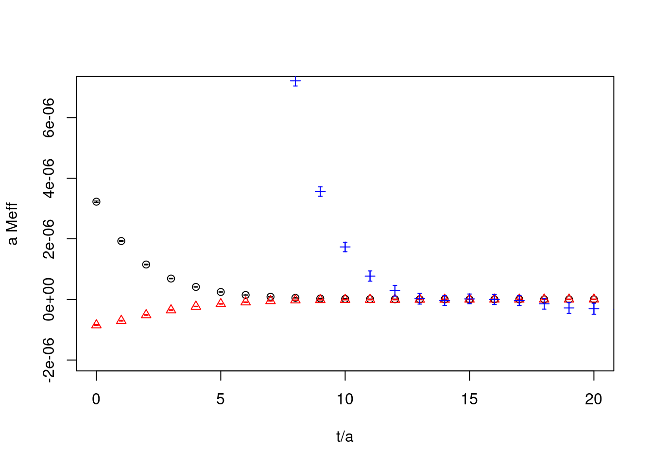
26.1.4 correlators
cor1 <- extractSingleCor.cf(cf=cfb, id=1)
#cor1.effmass <- bootstrap.effectivemass(cf=cor1)
cor2 <- extractSingleCor.cf(cf=cfb, id=2)
# cor2.effmass <- bootstrap.effectivemass(cf=cor2)
cor3 <- extractSingleCor.cf(cf=cfb, id=4)
# cor3.effmass <- bootstrap.effectivemass(cf=cor3)
plot(cor1, ylab="a Meff", xlab="t/a", col="black", xlim=c(0,20),ylim=c(-2e-6,7e-6))
plot(cor2, rep=TRUE, col="red",pch=2)
plot(cor3, rep=TRUE, col="blue",pch=3)