10.5 Power test using randomly drawn normally-distributed data that follows certain assumptions regarding mean differences
In the following procedure, we want to a-priori assess the required sample size for a statistical test of mean differences in two independent groups.
10.5.1 Preparing the function for your power test
In the following, we prepare a function that sets up our data and model for usage in another function that is called grid_search. grid_search uses that function to draw a specified amount of new samples.
The code demonstrates a sampling procedure that also included lavaan::cfa for specifying and analyzing the data.
We want to automate the procedure discussed in the previous chapters to randomize data repeatedly, to analyze the factor structure, and see how often a random sample of ‘n’ actually results in a significant mean difference between the latent variable in the two groups based on our assumptions concerning the data.
The function can be seen in the code block below.
#write function
function_test <- function(simNum, #this can be understood as the ID for each run of the function
                      n, # the sample size that gets varied
                      r, # the correlation between the items
                      m1, # the means of the indicators in group1
                      m2  # the means of the indicators in group1
                      ) {
#the covariance matrix that in this case of a standard normal distribution is a correlation matrix
R <- matrix(c(1, r, r, r,
              r, 1, r, r,
              r ,r, 1, r,
              r, r, r, 1),
            nrow = 4, ncol = 4)
# generate the two data sets
# be aware to make sure to call the right function from its respective package using "::"
test_norm1 <- as.data.frame(mvtnorm::rmvnorm(n, mean = c(m1,m1,m1,m1), sigma = R))
test_norm2 <- as.data.frame(mvtnorm::rmvnorm(n, mean = c(m2,m2,m2,m2), sigma = R))
# assining group values
test_norm1$group <- 1
test_norm2$group <- 2
# merge the two data sets
data <- as.data.frame(rbind(test_norm1, test_norm2))
# specify measurement model of the latent factor
model <- 'v =~ V1+V2+V3+V4

# label means

v ~ c(mean_1, mean_2)*1

# parameter for mean difference test

mean_diff := mean_2 - mean_1
'
# estimate the model
fit_model <- lavaan::cfa(model, data, meanstructure=T, group = "group", group.equal = c("loadings", "intercepts"))
# save parameter estimates
ests <- lavaan::parameterEstimates(fit_model)
# extract the relevant parameters
est <- ests[ests$label == 'mean_diff', 'est']
p <- ests[ests$label == 'mean_diff', 'pvalue']
    return(c(est = est,
           p = p,
           sig = (p < .05)))
}
10.5.2 Run the function of your power test with the desired specifications
We now call our new function inside grid_search and insert the necessary parameters. In the code block below (using the example of the first grid_search, see the comments in the code block below), we want to have an n that ranges from 10 to 500 with increments of 10, i.e., 10,20,30,40… and so on. The inter-item-correlations are set to $r = .25$. The means are m1 = 0 and m2 = 0.2 for group 1 and group 2, respectively.
With n.iter the function repeatedly draws a random sample of our choosing and fit the model for the parameters set above. That means that for n.iter = 1000 there are 1000 drawn samples for each parameter set.
The specifications below lead to 50.000 repetitions for each test run (i.e, 200.000 runs altogether), which will take a while to run.
The results from each run will be saved to an Rda. file.
# first, we record the starting time, to get an idea how long our test will take
start_time <- Sys.time()
# then we call the function grid_search for our function_test where r = .25 and save the results to 'power25'
power25_md2 <- grid_search(
  func = function_test,
  params = list(n = seq(10, 500, by = 10)), # increments of n
  r = .25, # inter-item-correlation
  m1 = 0, # mean for the observed variables of group 1
  m2 = 0.2, #  mean for the observed variables of group 2
  n.iter = 1000, # repetitions for each parameter set.
  output = 'data.frame', # save output to a dataframe
  parallel='snow',
  ncpus=4 # how many cpus will get used, my max. is 4
  )
# record the time again and see how long the first test performed
end_time1 <- Sys.time()
end_time1 - start_time

#we call the function grid_search for our function_test where r = .5 and save the results to 'power50'
power50_md2 <- grid_search(
  func = function_test,
  params = list(n = seq(10, 500, by = 10)),
  r = .5,
  m1 = 0,
  m2 = 0.2,
  n.iter = 1000,
  output = 'data.frame',
  parallel='snow',
  ncpus=4
  )

# we call the function grid_search for our function_test where r = .8 and save the results to 'power80'
power80_md2 <- grid_search(
  func = function_test,
  params = list(n = seq(10, 500, by = 10)),
  r = .8,
  m1 = 0,
  m2 = 0.2,
  n.iter = 1000,
  output = 'data.frame',
  parallel='snow',
  ncpus=4
  )

# we call the function grid_search for our function_test where r = .99 and save the results to 'power99'
power99_md2 <- grid_search(
  func = function_test,
  params = list(n = seq(10, 500, by = 10)),
  r = 0.99,
  m1 = 0,
  m2 = 0.2,
  n.iter = 1000,
  output = 'data.frame',
  parallel='snow',
  ncpus=4
  )

end_time2 <- Sys.time()
end_time2 - start_timesave(power25_md2, file="power25_md2.RData")
save(power50_md2, file="power50_md2.RData")
save(power80_md2, file="power80_md2.RData")
save(power99_md2, file="power99_md2.RData")10.5.3 Display and interpret the results
Afterward, we would like to visualize the results with the code below.
#combine the data output
(result_power_diff <- results(power25_md2) %>%
    mutate(corr = "R1: r = .25") %>%
      bind_rows(results(power50_md2) %>%
      mutate(corr = "R2: r = .5")) %>%
          bind_rows(results(power80_md2) %>%
          mutate(corr = "R3: r = .8")) %>%
            bind_rows(results(power99_md2) %>%
            mutate(corr = "R4: r = .99")) %>%
    group_by(corr, n.test) %>%
    summarise(power=mean(sig, na.rm=TRUE)))

#display results
(img_diff <- result_power_diff %>%
  ggplot(., aes(x = n.test,
                y = power,
                color = factor(corr))) +
  geom_point() +
  scale_x_continuous(breaks = seq(0, 500, by = 50))) +
  geom_smooth(se = F) +
  geom_hline(yintercept = .80, linetype = "dashed") +
  geom_hline(yintercept = .95, linetype = "dashed") +
  theme_bw() +
  labs (x = "sample size",
        y = "power",
        color = "Latent mean difference of .2")
The visual representation of the results looks as follows.
## # A tibble: 200 x 3
## # Groups:   corr [4]
##    corr        n.test  power
##    <chr>        <dbl>  <dbl>
##  1 R1: r = .25     10 0.0896
##  2 R1: r = .25     20 0.142
##  3 R1: r = .25     30 0.141
##  4 R1: r = .25     40 0.204
##  5 R1: r = .25     50 0.261
##  6 R1: r = .25     60 0.318
##  7 R1: r = .25     70 0.384
##  8 R1: r = .25     80 0.447
##  9 R1: r = .25     90 0.497
## 10 R1: r = .25    100 0.544
## # ... with 190 more rows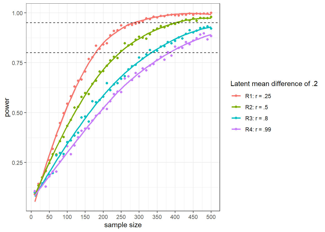
The results may appear surprising at first sight. However, as the latent factor has a higher variance in R4 (Variance = .99) than in R1 (Variance = .25), the effect size is smaller in R4 (effect size = .2) than in R1 (effect size = .8). Consequently, with the smaller effect size, you would need more observations to detect the smaller effect.
If you want to adjust for effect size, this will entail using different means with the different variances, and the results would differ accordingly.