Chapter 16 Analyzing Text Data
Hello! Today, we’ll be working primarily with the tidytext package, a great beginner package for learning NLP in R.
options(scipen=999) #use this to remove scientific notation
#packages <- c("tidytext", "tokenizers", "wordcloud", "textdata")
#install.packages(packages)
library(tidyverse)
library(tidytext)
library(tokenizers)
library(wordcloud)
library(textdata)
This week, we’ll work with the academictwitter data that we used in the iterations chapter
twitter_data <- read_csv("data/rtweet_academictwitter_2021.csv")
#variable.names(twitter_data) #get a list of all the variable names
#str(twitter_data)

tw_data <- twitter_data %>%
  select(status_id, created_at, screen_name, text)
The main variable we’ll be working with is text, which contains the tweets themselves. We can use head() to look at the first few
## [1] "Please, always use a #colorblind friendly palette when drawing figures, especially when colours are important to distinguish points/regions. If I could I'd recolour all my previous figures. @AcademicChatter\r\n#academicchatter #AcademicTwitter https://t.co/zfzkEkvvyy"
## [2] "This is a sad development: #JSTOR will move to stop hosting current articles and go back to only archival issues. #AcademicTwitter \r\n\r\nhttps://t.co/zIhRgfPHoW"
## [3] "The Journal of Sports Sciences is seeking an academic researcher with a strong research background in #sportscience. Apply to become the Social Media Editor of the journal before January 31: https://t.co/RBNicyj6nj #AcademicTwitter @JSportsSci @grantabt https://t.co/xXPoG5v9y8"
## [4] "Hear what a participant had to say about our workshop last week!<U+0001F9E1><U+0001F9E1><U+0001F9E1> theres still time to book your ticket! Follow the link https://t.co/oVNh7PSPT5 @MaryCParker #antiracism #antiracist #AcademicTwitter #virtuallearning #education https://t.co/PMhAJA9SRo"
## [5] "Please, always use a #colorblind friendly palette when drawing figures, especially when colours are important to distinguish points/regions. If I could I'd recolour all my previous figures. @AcademicChatter\r\n#academicchatter #AcademicTwitter https://t.co/zfzkEkvvyy"
16.1 str_replace_all()
You’ll notice that one of the tweets (#4) contains some extra character encodings (\r\n\r\n). We can use a function you may have seen before, str_replace_all() in the stringr package, to remove these encodings. This function allows you to replace a substring pattern with another pattern. So, for example, if you have a string that said, “Author: John Smith” and you wanted to replace the “Author:” part with “Byline -”, you could use str_replace_all(character vector, "Author:", "Byline - "). Note that str_replace_all() takes three arguments: (1) the character vector/variable, (2) the string you want to replace, and (3) a replacement string. If you wanted to replace a string with nothing, you could use "".
tw_data$text <- str_replace_all(tw_data$text, "\\\r", " ") %>%
  str_replace_all("\\\n", " ")

head(tw_data$text, 5)
## [1] "Please, always use a #colorblind friendly palette when drawing figures, especially when colours are important to distinguish points/regions. If I could I'd recolour all my previous figures. @AcademicChatter #academicchatter #AcademicTwitter https://t.co/zfzkEkvvyy"
## [2] "This is a sad development: #JSTOR will move to stop hosting current articles and go back to only archival issues. #AcademicTwitter https://t.co/zIhRgfPHoW"
## [3] "The Journal of Sports Sciences is seeking an academic researcher with a strong research background in #sportscience. Apply to become the Social Media Editor of the journal before January 31: https://t.co/RBNicyj6nj #AcademicTwitter @JSportsSci @grantabt https://t.co/xXPoG5v9y8"
## [4] "Hear what a participant had to say about our workshop last week!<U+0001F9E1><U+0001F9E1><U+0001F9E1> theres still time to book your ticket! Follow the link https://t.co/oVNh7PSPT5 @MaryCParker #antiracism #antiracist #AcademicTwitter #virtuallearning #education https://t.co/PMhAJA9SRo"
## [5] "Please, always use a #colorblind friendly palette when drawing figures, especially when colours are important to distinguish points/regions. If I could I'd recolour all my previous figures. @AcademicChatter #academicchatter #AcademicTwitter https://t.co/zfzkEkvvyy"Why did we use \\\ instead of just one \? \ is actually a special character that is used to identify other language patterns. When we use stringr or one of the base R packages to search for substrings, we can use “regular expressions” to find substring patterns (rather than exact patterns). For example, say you wanted to delete all the urls in your text file, but some of them started as “http://” while others started as “https://”. You can use regular expressions that can consider both language patterns! Learn more about regular expressions here, or refer back to our lesson on Week 6.
Let’s go ahead and remove the urls now. Notice that each URL has its own shortened identifier (e.g., HYf8726AaV vs. H10maACu2H). We therefore will need a regular expression that can account for tihs variety across the dataset.
#tw_data$text[1] #what does the first row look like?
str_replace_all(tw_data$text[1], "https://t.co/", "") #replaces the substring pattern in the first tweet, does not save the result
## [1] "Please, always use a #colorblind friendly palette when drawing figures, especially when colours are important to distinguish points/regions. If I could I'd recolour all my previous figures. @AcademicChatter #academicchatter #AcademicTwitter zfzkEkvvyy"With the line above, we’ve figured out the substring that will likely be the same across the whole dataset. That brings up half of the way there! But how do we handle the characters that change? We could use the \\S character pattern, which represents everything expect a space. One thing you may have noticed is that the urls have 10 characters in its identifiers. So, you could use \\S ten times.
## [1] "Please, always use a #colorblind friendly palette when drawing figures, especially when colours are important to distinguish points/regions. If I could I'd recolour all my previous figures. @AcademicChatter #academicchatter #AcademicTwitter "Or, you can use a quantifier to indicate the number of times you want the character before to repeat.
## [1] "Please, always use a #colorblind friendly palette when drawing figures, especially when colours are important to distinguish points/regions. If I could I'd recolour all my previous figures. @AcademicChatter #academicchatter #AcademicTwitter "Looks like we have constructed the right substring pattern! One thing you may have noticed is that the tweet has a space at the end. This is the space between the last word and the URL link. If you would like to remove this, put a space in front of the substring search (" https://t.co/\\S{10}").
Now, let’s apply this to all the tweets.
If you View() the dataset now, you’ll notice that the text column does not have tweets. In the next steps, we’ll learn about other ways to remove things from and process text data.
16.2 Data Processing
Compared to numbers, text data is complex. A computer can understand how to add the number 4 to the number 5, but (without you providing instructions), a computer cannot tell how many the words in string, “good morning, how are you?” (There are five.) For a computer to identify words, you have to tell R how to “parse” text (i.e., break down a string into its linguistic parts).
The most common way you parse text data is using a process called “tokenizing,” where you treat each word as a “token.” You can also tokenize sentences, which results in sentence tokens. To tokenize, we’ll use unnest_tokens() in the tidytext pakage. unnest_tokens() takes three arguments: the dataset, the output variable you want to create (we’ll use “words”) and the character variable you want to tokenize (the “input”). By default, the unnest_tokens() will tokenize by “words”, but you can also parse by “ngrams”, “sentences”, “paragraphs” and more. There are also other useful arguments, like to_lower, which converts all the tokens into lower-case.
tweet_tokenized <- tw_data %>% unnest_tokens(word, text, to_lower = TRUE)
head(tweet_tokenized$word, 13) #shows the first 10 words in the dataset
## [1] "please" "always" "use" "a" "colorblind" "friendly" "palette" "when" "drawing" "figures" "especially" "when"
## [13] "colours"## [1] "Please, always use a #colorblind friendly palette when drawing figures, especially when colours are important to distinguish points/regions. If I could I'd recolour all my previous figures. @AcademicChatter #academicchatter #AcademicTwitter"Notice that, when you look at the first 13 words of the tokenized dataset (tidy_tweets), these are the words in the first tweet. In addition to transforming the sentence into its word tokens, the function also converted all the text to lower-case, using the to_lower() function.
16.2.1 Stopwords
One of the first steps in NLP processing is to remove words that do not contain a lot of information, but occur frequently in a corpus (a collection of linguistic messages). To do so, computational scholars use “stop words” lists, or lists of words we want to exclude from our analysis. Learn more about stop words from the Wikipedia page here.
Thankfully, tidytext has some preset stop words. We can tweak these dictionaries to tailor them to our needs and our data’s needs.
## # A tibble: 1,149 x 2
##    word        lexicon
##    <chr>       <chr>
##  1 a           SMART
##  2 a's         SMART
##  3 able        SMART
##  4 about       SMART
##  5 above       SMART
##  6 according   SMART
##  7 accordingly SMART
##  8 across      SMART
##  9 actually    SMART
## 10 after       SMART
## # i 1,139 more rows
We can add words to this stop words list by creating a data frame with custom stop words. You can then rbind() your custom list of words to the preset list of stop words.
final_stop <- data.frame(word = c("said", "u", "academictwitter"), lexicon = "custom") %>%
  #we're going to create a new dataframe with custom words
  rbind(stop_words) #then, we rbind() them to the original dictionary
To remove this list of stopwords, custom or original, we’ll use the anti_join() function.
## Joining, by = "word"## [1] "colorblind" "friendly" "palette" "drawing" "figures" "colours" "distinguish" "regions"
## [9] "recolour" "previous" "figures" "academicchatter" "academicchatter"Notice that stop words like “i” and “to” have been removed. Many of the words in a stopwords list include things like function words.
What are the most common words in the document?
## # A tibble: 18,584 x 2
##    word                n
##    <chr>           <int>
##  1 academicchatter  8855
##  2 phdchat          4274
##  3 phd              3633
##  4 amp              2172
##  5 academic         2050
##  6 openacademics    1988
##  7 phdlife          1733
##  8 research         1720
##  9 time             1566
## 10 dm               1447
## # i 18,574 more rows
# we use dplyr:: first because we are telling R we want to use the count function in the dplyr package.We can also display this graphically!
tweet_tokenized %>%
  dplyr::count(word, sort = TRUE) %>% #let's count the top words in our list
  filter(n > 1500) %>%    #only considers words used  more than 15,000 times
  mutate(word = reorder(word, n)) %>% #orders the words by it's frequency (n), not alphabetically
  ggplot(aes(word, n)) + #you can pipe in a ggplot!
  geom_col() + #the geom!
  coord_flip() #make the bars horizontal
16.2.2 Wordclouds
Now that we have these word-tokens, we can also visualize these results as a word cloud! To do this, we’ll use the wordcloud() function in the wordcloud package.
tweet_tokenized %>%
  dplyr::count(word, sort = TRUE) %>% #construct a count of the top words in R
  with(wordcloud(word, n, max.words = 100)) #makes a word cloud of the top 100 words
## Warning in wordcloud(word, n, max.words = 100): academicchatter could not be fit on page. It will not be plotted.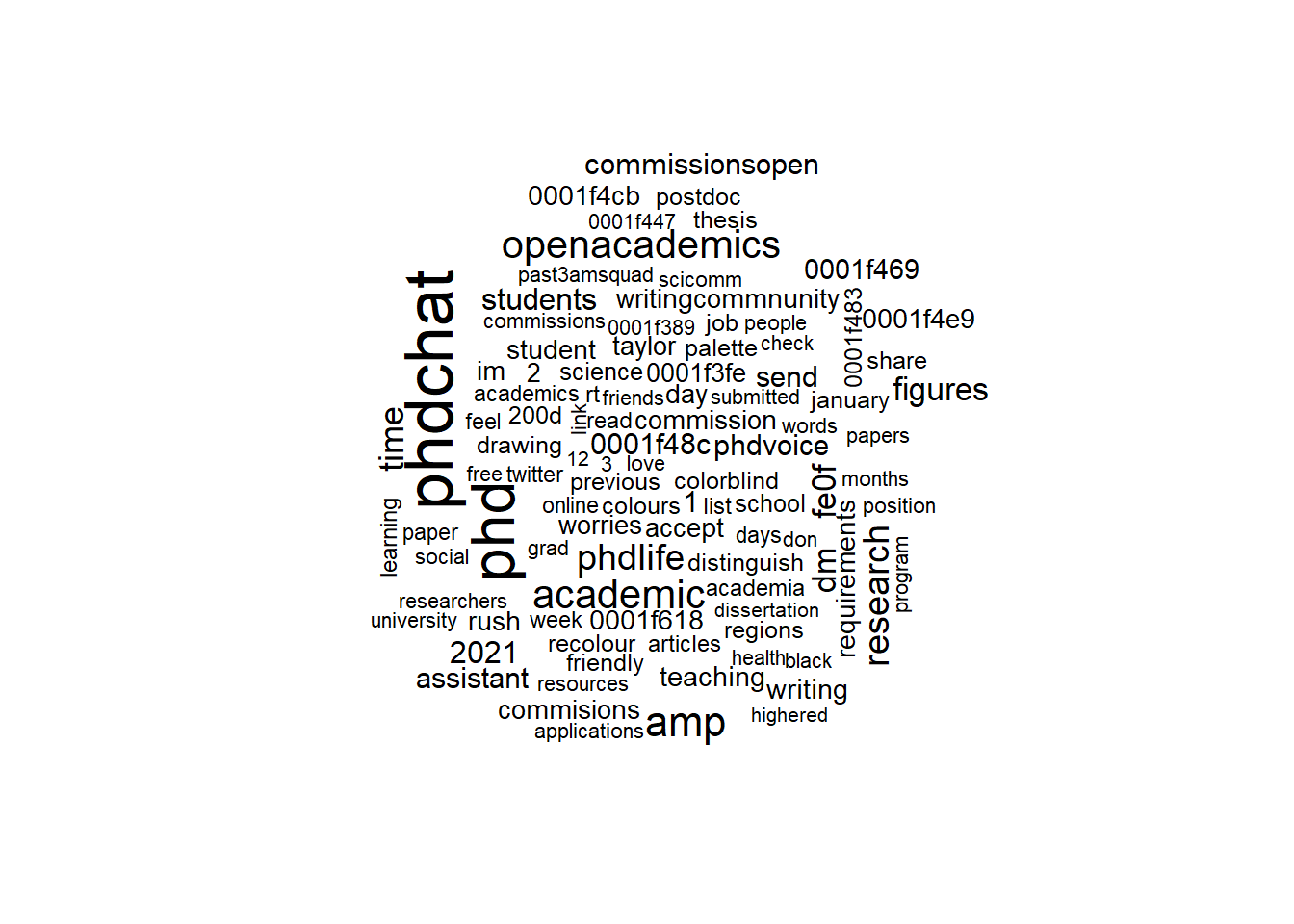
As we can see, the most frequent words (like phdchat, phd, and academic) are the largest. Note that you may also get a warning that extra large words (like academicchatter) may not appear due to size issues. If you wanted to force the keyword in, you could adjust the scale of the wordcloud (see here for more).
16.3 Dictionary analysis
16.3.1 Sentiment dictionaries
Thus far, we have used a list of words to remove word-tokens from the corpus (the stop words list). We can also treat a list of words as a dictionary. Dictionaries are lists of keywords that reflect some sort of concept (e.g., sentiment, emotion, bias, etc). While simple, dictionary methods can be incredibly useful. Sometimes, we aggregate coded words to the message-level.
One popular type of dictionary is the sentiment dictionary. Sentiment dictionaries are list of words representing positive or negative sentiment. In textdata, there are three main sentiment dictionaries:
1. AFINN - In this dictionary, positive and negative words are labeled on a spectrum from -5 (most negative) to +5 (most positive)
2. bing- In this dictionary, words can be labeled positive OR negative
3. nrc- In this dictionary, words are labeled by a discrete emotion, like fear or joy
If you check out ?get_sentiments (which we will discuss below), you’ll notice there is actually a fourth dictionary (loughran). This one is similar to bing in that each word is labeled positive or negative, but it was specifically constructed for finance documents.
I encourage you to check all these dictionaries out, but we’ll use AFINN for this tutorial.
To call this dictionary, we’ll use the get_sentiments() function (note that there is an s in get_sentiments). This tidytext function allows you to get a specific dictionary from the textdata package.
afinn_dictionary <- get_sentiments("afinn")

head(afinn_dictionary, 10) #let's look at the first 10 words of this dictionary
## # A tibble: 10 x 2
## word value
## <chr> <dbl>
## 1 abandon -2
## 2 abandoned -2
## 3 abandons -2
## 4 abducted -2
## 5 abduction -2
## 6 abductions -2
## 7 abhor -3
## 8 abhorred -3
## 9 abhorrent -3
## 10 abhors -3Now that we have our dictionary, let’s apply it! To do this, we’ll use the join function inner_join() from dplyr. inner_join() is a specialized join function (the family of join functions allow you to combine two data frames). Learn more about inner_join here and here.
word_counts_senti <- tweet_tokenized %>% #we're going to use our tokenized data frame
  inner_join(afinn_dictionary) #attach the afinn dictionary to it
## Joining, by = "word"If a word is not attached to a sentiment, it is excluded (if you would like to include it, you could use the full_join() function, also in dplyr).
Does the data frame have the merged content? One thing you’ll notice is that word_counts_senti has a new varaible (value). Let’s check this variable out
## # A tibble: 6 x 5
##   status_id created_at          screen_name     word     value
##       <dbl> <dttm>              <chr>           <chr>    <dbl>
## 1   1.35e18 2021-01-15 17:33:32 stevebagley     friendly     2
## 2   1.35e18 2021-01-15 17:33:31 Canadian_Errant sad         -2
## 3   1.35e18 2021-01-15 17:33:31 Canadian_Errant stop        -1
## 4   1.35e18 2021-01-15 17:33:21 DebSkinstad     strong       2
## 5   1.35e18 2021-01-15 17:32:23 ucdavisSOMA     friendly     2
## 6   1.35e18 2021-01-15 17:31:42 ChemMtp         bad         -3
As we can see, the data frame word_counts_senti contains the all the variables in tweet_tokenized and the value variable from the afinn dictionary.
We can construct a sentiment variable for each tweet by taking the cumulative sum of all the sentiments.
tweet_senti <- word_counts_senti |>
  dplyr::group_by(status_id) |>
  dplyr::summarize(sentiment = sum(value))

head(tweet_senti)
## # A tibble: 6 x 2
## status_id sentiment
## <dbl> <dbl>
## 1 1.35e18 4
## 2 1.35e18 4
## 3 1.35e18 1
## 4 1.35e18 4
## 5 1.35e18 -2
## 6 1.35e18 -3As you see with the head() function, the data frame tweet_senti produces a data frame with two columns: the status_id and the sentiment, which is the sum of all the sentiment words. A tweet scored as -10, like the first tweet, would be quite negative. But we don’t know this for sure with the data frame. We need to merge this data frame with the message-level data frame (tw_data).
tw_data <- tw_data %>% #let's take our message-level data frame
  full_join(tweet_senti) #and add the variables from tweet_senti
## Joining, by = "status_id"Importantly, not all tweets have a word from the sentiment dictionary. summary() would tell us that there are 13,328 such tweets. We call fill these tweets with zero.
##    Min. 1st Qu.  Median    Mean 3rd Qu.    Max.    NA's
## -16.000 -1.000 1.000 1.133 3.000 19.000 7547tw_data$sentiment[is.na(tw_data$sentiment)] <- 0 #if tw_data$sentiment is NA, replace with 0
summary(tw_data$sentiment) #nore that the NA's information disappears, because there are no NAs in the variable## Min. 1st Qu. Median Mean 3rd Qu. Max.
## -16.0000 0.0000 0.0000 0.7091 2.0000 19.0000##
## -16 -15 -14 -12 -11 -10 -9 -8 -7 -6 -5 -4 -3 -2 -1 0 1 2 3 4 5 6 7 8 9 10 11 12 13 14 15 16
## 2 1 2 3 15 29 8 19 22 119 83 354 421 1304 1166 8207 2503 2720 1208 814 399 293 154 168 70 31 24 11 6 6 1 8
## 17 19
## 5 6When we use table(), we can see that the range of sentiment is from -16 to 19. What does the most negative and most positive tweets look like?
## # A tibble: 3 x 1
## text
## <chr>
## 1 "She was just getting on a flt & pp were chanting \ufffdTrump\ufffd<U+0001F440> Students thought they were going to TUSDM but run in to Path liar @TuftsD~
## 2 "#FirstWorldIssues alert. I miss complaining about bad coffee & bad food served at academic conferences.I even miss complaining about how bad the WiFi is a~
## 3 "#FirstWorldIssues alert. I miss complaining about bad coffee & bad food served at academic conferences.I even miss complaining about how bad the WiFi is a~## # A tibble: 6 x 1
## text
## <chr>
## 1 A wonderful opportunity to submit your work (esp for ECRs) and have the opportunity to win the @PublicAnthropol award. Journal edited by my brilliant colleague ~
## 2 A wonderful opportunity to submit your work (esp for ECRs) and have the opportunity to win the @PublicAnthropol award. Journal edited by my brilliant colleague ~
## 3 A wonderful opportunity to submit your work (esp for ECRs) and have the opportunity to win the @PublicAnthropol award. Journal edited by my brilliant colleague ~
## 4 A wonderful opportunity to submit your work (esp for ECRs) and have the opportunity to win the @PublicAnthropol award. Journal edited by my brilliant colleague ~
## 5 A wonderful opportunity to submit your work (esp for ECRs) and have the opportunity to win the @PublicAnthropol award. Journal edited by my brilliant colleague ~
## 6 A wonderful opportunity to submit your work (esp for ECRs) and have the opportunity to win the @PublicAnthropol award. Journal edited by my brilliant colleague ~With the most negative tweet, word that probably produced a highly negative sentiment for the tweets included bad, fraud, and threats.
How negative are these words?
## # A tibble: 1 x 2
##   word  value
##   <chr> <dbl>
## 1 fraud -4## # A tibble: 1 x 2
## word value
## <chr> <dbl>
## 1 bad -3## # A tibble: 1 x 2
## word value
## <chr> <dbl>
## 1 threats -2On the flip side, the positve tweet appears to be a repeat of the same tweet 6 times, containing positive keywords like wonderful and brilliant.
## # A tibble: 1 x 2
##   word      value
##   <chr>     <dbl>
## 1 wonderful 4## # A tibble: 1 x 2
## word value
## <chr> <dbl>
## 1 brilliant 4If we check the dictionary, we can see that both wonderful and brillaint have a sentiment score of +4.
However, there are serious limitations to this approach: dictionary methods cannot account for negations, like “not wonderful,” for example.
Want to construct wordclouds based on sentiment? Check out this tutorial.
16.3.2 Custom building
But what if you wanted to create your own dictionary? Perhaps we just wanted the tweets mentioning a candidate (Biden, Trump, Pence, or Harris). Let’s construct this dictionary now.
phd_dictionary <- data.frame(word = c("phdchatter", "phd", "dissertating", "dissertation"),
                             phd = c("phd", "phd", "phd", "phd"))
We can then use inner_join(), just as we did with the afinn dictionary, to test this dictionary.
candidate_count_senti <- tweet_tokenized %>%
  inner_join(phd_dictionary) #attach the candidate_dictionary to it
## Joining, by = "word"How many tweets used a PhD word?
subset(candidate_count_senti, phd == "phd") %>% #subsets all words where a Rep is mentioned
  distinct(status_id) %>% #you can use distinct() to remove status_id duplicates
  nrow() #get the number of rows of this data frame
## [1] 3413What if we wanted to re-combine these results with the broader dataset (tw_data)? Unlike value in the afinn dictionary, party is not a numeric. But it is categorical: a PhD word was mentioned (or not)
phd_tweets <- subset(candidate_count_senti, phd == "phd") %>%
  distinct(status_id) #returns a data frame with one variable, status_id
phd_tweets$phd <- TRUE #creates a new variable in phd_tweets called "phd" which contains information about whether there was a Ph.D keyword or not.

tw_data <- tw_data %>%
  full_join(phd_tweets)
## Joining, by = "status_id"You’ll now notic that tw_data has two new variables Dem and Rep.
## [1] 6## [1] "status_id" "created_at" "screen_name" "text" "sentiment" "phd"What does this data frame look like?
## [1] NA NA NA NA NA NA NA NA NA NAAs you can see, tweets mentioning a Ph.D word are coded as TRUE. But tweets not mentioning a Ph>D word are not FALSE, they are NA. Let’s fix that.
## [1] FALSE FALSE FALSE FALSE FALSE FALSE FALSE FALSE FALSE FALSEOn average, do tweets mentioning a Ph.D word have a higher or lower sentiment than tweets not mentioning a Ph.D word?
## # A tibble: 1 x 1
##   `mean(sentiment, na.rm = TRUE)`
##                             <dbl>
## 1 0.433## # A tibble: 1 x 1
## `mean(sentiment, na.rm = TRUE)`
## <dbl>
## 1 0.765Based on this analysis, we see that tweets mentioning Republicans has an average sentiment score of 0.432,while tweets mentioning Democrats has an average sentiment score of 0.765.
16.4 n-gram analysis
The last thing we’ll cover in this tutorial is an n-gram analysis. An n-gram analysis allows you to study a sequence of words. Two words in a sequence, like “Republican Party”, is a bigram. Three words in a sequence, like “Department of Justice”, is a trigram. A 5-gram (quintgram) would have 5 consecutive words (e.g., “President of the United States”)
To do a bigram analysis, we’ll use the unnest_token() function. Previously, we wanted word tokens. But if we wanted ngrams, we can set the token argument to “ngram”. We can also add the n argument, which tells R how long your ngram should be (if n = 3, you would be looking for trigrams).
What does this data frame look like?
## # A tibble: 6 x 6
##   status_id created_at          screen_name sentiment phd   bigram
##       <dbl> <dttm>              <chr>           <dbl> <lgl> <chr>
## 1   1.35e18 2021-01-15 17:33:32 stevebagley         2 FALSE please always
## 2   1.35e18 2021-01-15 17:33:32 stevebagley         2 FALSE always use
## 3   1.35e18 2021-01-15 17:33:32 stevebagley         2 FALSE use a
## 4   1.35e18 2021-01-15 17:33:32 stevebagley         2 FALSE a colorblind
## 5   1.35e18 2021-01-15 17:33:32 stevebagley         2 FALSE colorblind friendly
## 6   1.35e18 2021-01-15 17:33:32 stevebagley         2 FALSE friendly palette
Now, we have a bigram column. Yay! What are the most common bigrams?
## # A tibble: 20 x 2
##    bigram                              n
##    <chr>                           <int>
##  1 academictwitter academicchatter  3379
##  2 academicchatter academictwitter  3003
##  3 in the                           1458
##  4 u fe0f                           1410
##  5 academictwitter phdchat          1387
##  6 phdchat academictwitter          1231
##  7 if you                           1158
##  8 u 0001f48c                       1158
##  9 u 0001f469                       1018
## 10 a phd                             987
## 11 us a                              972
## 12 send us                           957
## 13 a dm                              952
## 14 s your                            952
## 15 no more                           947
## 16 academictwitter commissionsopen   944
## 17 commissionsopen commission        944
## 18 we got                            943
## 19 u u                               937
## 20 worries about                     937
While most of the bigrams appear to be hashtags, you may notice that we still have our stop words (like “if” and “a’). How do we remove bigrams with this combination? Well, we can use the separate() function in tidyr, which parses a character column based on a”delimiter” (in this case, the delimiter is a space). Learn more about delimiters here. We can then filter() out stop words. (filter() is a function in dplyr).
bigrams_separated <- tweet_bigram %>%
  separate(bigram, c("word1", "word2"), sep = " ")

tweet_biram_filtered <- bigrams_separated %>%
  filter(!word1 %in% final_stop$word) %>%
  filter(!word2 %in% final_stop$word) %>%
  unite(bigram, word1, word2, sep = " ")

tweet_biram_filtered %>%
  dplyr::count(bigram, sort = TRUE) %>%
  head(10)
## # A tibble: 10 x 2
## bigram n
## <chr> <int>
## 1 commissionsopen commission 944
## 2 accept rush 932
## 3 commisions writingcommnunity 932
## 4 commission commisions 932
## 5 im taylor 932
## 6 writingcommnunity academic 932
## 7 academicchatter academicchatter 777
## 8 colorblind friendly 708
## 9 drawing figures 702
## 10 figures academicchatter 702Interesting!
Want to visualize this bigram as a network? Check out this tutorial.
Want to make an ngram word cloud? Check out this tutorial.
A great tidytext run through by maintainer Julia Silge. Find it here.