Chapter 26 Quanteda
Hello fellow coders! Today, we’ll be going through the R package quanteda. Quanteda is a multi-purpose R package that has a lot of features for text analysis.
Quanteda Documentation here.
Quanteda Website here.
This week, we’ll be working with a dataset of tweets about ballot harvesting, Trump’s taxes, and SCOTUS. This is the same dataset we used in the tidytext tutorial
#setwd("")
#install.packages("quanteda")
library(tidyverse)
library(quanteda)

twitter_data <- read_csv("data/rtweet_academictwitter_2021.csv")
tw_data <- twitter_data %>%
  select(status_id, created_at, screen_name, text, source) #select our variables of interest
tw_data <- distinct(tw_data, status_id, .keep_all = TRUE) #remove status_id duplicates

tw_data$text <- str_replace_all(tw_data$text, "\\\r", " ") %>% #remove \r
  str_replace_all("\\\n", " ") %>% #removes \n
  str_replace_all(" https://t.co/\\S{10}", " ") %>% #removes url
  str_replace_all("<U+.{2,10}>", " ") #removes <U+______> encodings
26.1 Corpus Construction
A corpus is a collection (“library”) of text documents (or “files”, or “units of analysis”). Quanteda will convert a data frame to a corpus using the function corpus(). corpus() using one column as the “text”, and other columns as meta-data. Meta-data that are important to the corpus are called “docvars”. Meta-data that may help process the corpus faster, but are not actually part of the analysis, are called “metadoc”. Below, we use the docvars() function to create docvars for our corpus. But, you can also use the docvars argument in corpus().
tw_corpus <- corpus(tw_data$text,
                    docnames = tw_data$status_id) #designate the status_id file as the id of the tweet
docvars(tw_corpus, "screen_name") <- tw_data$screen_name
docvars(tw_corpus, "time") <- tw_data$created_at
docvars(tw_corpus, "source") <- tw_data$source

head(tw_data)
## # A tibble: 6 x 5
## status_id created_at screen_name text source
## <dbl> <dttm> <chr> <chr> <chr>
## 1 1.35e18 2021-01-15 17:33:32 stevebagley "Please, always use a #colorblind friendly palette when drawing figures, especially when colours are import~ Twitt~
## 2 1.35e18 2021-01-15 17:33:31 Canadian_Errant "This is a sad development: #JSTOR will move to stop hosting current articles and go back to only archival ~ Twitt~
## 3 1.35e18 2021-01-15 17:33:21 DebSkinstad "The Journal of Sports Sciences is seeking an academic researcher with a strong research background in #spo~ Twitt~
## 4 1.35e18 2021-01-15 17:32:55 aceofmine "Hear what a participant had to say about our workshop last week! theres still time to book your ticket!~ Twitt~
## 5 1.35e18 2021-01-15 17:32:23 ucdavisSOMA "Please, always use a #colorblind friendly palette when drawing figures, especially when colours are import~ Twitt~
## 6 1.35e18 2021-01-15 17:31:42 ChemMtp "When you have a bad day in lab, cannot get the desired results or don't understand something... #Academ~ Twitt~## [1] "corpus" "character"## Text Types Tokens Sentences screen_name time source
## 1 1350134035012587520 32 36 3 stevebagley 2021-01-15 17:33:32 Twitter for iPad
## 2 1350134027496415232 22 23 2 Canadian_Errant 2021-01-15 17:33:31 Twitter for Android
## 3 1350133988820742144 33 35 2 DebSkinstad 2021-01-15 17:33:21 Twitter for iPhone
## 4 1350133880104366080 28 30 3 aceofmine 2021-01-15 17:32:55 Twitter for iPhone
## 5 1350133743344730112 32 36 3 ucdavisSOMA 2021-01-15 17:32:23 Twitter for iPhone
## 6 1350133571265171456 20 22 2 ChemMtp 2021-01-15 17:31:42 Twitter for AndroidWith class(), you can tell that your new object tw_corpus is a corpus-type. With summary(), we can see that this corpus contains a Text variable (this identifies the tweet), a Types variable (the number of words), a Tokens variable (the number of unique words), and a Sentences variable (the number of sentences in the message). You will also see our docvars (status_id, screen_name, and time).
26.1.1 Subsetting Corpus
You can subset your corpus by the docvars features. For example, let’s summarize the corpus for just Fox News articles.
##                  Text Types Tokens Sentences     screen_name                time              source
## 1 1350134035012587520    32     36         3     stevebagley 2021-01-15 17:33:32    Twitter for iPad
## 2 1350134027496415232    22     23         2 Canadian_Errant 2021-01-15 17:33:31 Twitter for Android
## 3 1350133988820742144    33     35         2     DebSkinstad 2021-01-15 17:33:21  Twitter for iPhone
## 4 1350133880104366080    28     30         3       aceofmine 2021-01-15 17:32:55  Twitter for iPhone
## 5 1350133743344730112    32     36         3     ucdavisSOMA 2021-01-15 17:32:23  Twitter for iPhone
## 6 1350133571265171456    20     22         2         ChemMtp 2021-01-15 17:31:42 Twitter for Android
## 7 1349311705965277184 13 15 1 ChemMtp 2021-01-13 11:05:54 Twitter for Android
## 8 1350133536129478656 30 32 2 FOW_Researcher 2021-01-15 17:31:33 Tweetbot for i<U+039F>S
## 9 1349029477242839040 40 43 2 Liar_RKasberg 2021-01-12 16:24:25 Twitter for iPhone
## 10 1349822898018553856 31 31 1 Liar_RKasberg 2021-01-14 20:57:12 Twitter for iPhoneIn the above, we subset tw_corpus by tweets that are posted on September 24, 2020 and after.
26.2 Tokenizing
If you remember from our tidytext tutorial, “tokenizing” refers to the breaking down of a document (in this case, an article) into it words (called “tokens”). To tokenize using quanteda, we can use the token function, which also allows you to remove symbols, punctuations, hyphens, urls, and twitter features (which transforms hashtags into normal word-tokens).
Like unnest_tokens() in tidytext, The quanteda package’s token() function also allows you to treat a sentence as a token, rather than a word, and has an ngram attribute, which allows you to treat a bigram (or more) as a token. Although you can pass a character list, I would recommend tokenizing an already-processed corpus, since it will also attach the meta-data to your tokens.
Learn more about tokens here. As of quanteda 3.0, tokenizing is an essential step before proceeding with a lot of other analyses.
#?tokens #learn more about tokens with the help function

tw_tokens <- tokens(tw_corpus)
tw_corpus[1] #let's see the first tweet
## Corpus consisting of 1 document and 3 docvars.
## 1350134035012587520 :
## "Please, always use a #colorblind friendly palette when drawi..."## Tokens consisting of 1 document and 3 docvars.
## 1350134035012587520 :
## [1] "Please" "," "always" "use" "a" "#colorblind" "friendly" "palette" "when" "drawing" "figures"
## [12] ","
## [ ... and 24 more ]Let’s see what this looks like at the sentence-level. To make sure we tokenize by sentence, we’ll need to modify the what argument (which defaults to “word”).
## Corpus consisting of 1 document and 3 docvars.
## 1350133880104366080 :
## "Hear what a participant had to say about our workshop last w..."## Tokens consisting of 1 document and 3 docvars.
## 1350133880104366080 :
## [1] "Hear what a participant had to say about our workshop last week!"
## [2] "theres still time to book your ticket!"
## [3] "Follow the link @MaryCParker #antiracism #antiracist #AcademicTwitter #virtuallearning #education"Most tweets are only one sentence. But with newspaper articles, press releases, and even longer social media posts (like Facebook posts), this can be very useful
26.2.1 Stopwords
One thing you may have realized is that we have not applied any stopwords, as we did with tidytext. Aside from those keywords, we can also use stop words from the stopwords package. This stopwords package contains stopwords for multiple languages. For more, see this link: https://github.com/stopwords-iso/stopwords-iso (or write ?stopwords) in the console.
In quanteda, you can remove stopwords using the tokens_remove() function. However, you can also process the tokens in other ways, using remove_ attributes in the tokens() function. Belowe, we remove punctuations (remove_punct), symbols (remove_symbols), numbers (remove_numbers), urls (remove_url)
#install.packages("stopwords")
tw_token_clean <- tokens(tw_corpus,
                 remove_punct = TRUE,
                 remove_symbols = TRUE,
                 remove_numbers = TRUE,
                 remove_url = TRUE,
                 remove_separators = TRUE) %>% #check out ?tokens for more
  tokens_remove(stopwords("en")) #remove stopwords with the token_remove() function
#also try out stopwords(source = "smart")!
Even with the removal of the preset stopwords, there may still be more words we want to remove (e.g., “s”). We can do so by creating a custom stopword list, and joining it to the preset stopword list.
26.2.2 KWIC
KWIC stands for “KeyWord in Context”, which is a common term in corpus linguistics. KWIC analyses are most common in “concordance” analyses, where the order of the words are retained. This allows the researcher to identify a keyword of interest, and see that word in its context (that is, the 5 words before and after it).
The function kwic() is quanteda’s iteration of this. Let’s see the word “dissertation” in context. To make sure we capture “dissertation” and “Dissertation”, you can set the optional argument case_insensitive to TRUE.
texas_kwic <- kwic(tw_token_clean, pattern = "dissertation", case_insensitive = TRUE)
nrow(texas_kwic)
## [1] 362## Keyword-in-context with 10 matches.
## [1349892660174200832, 7] beloved wife@jorellanalvear defend PhD | dissertation | @Uni_MR@LCRS_UniMR long journey together
## [1349011466456805376, 2] Defended | dissertation | yesterday Hit daily activity goal
## [1349009298710552576, 5] told advisor wrote sentences | dissertation | today despite trying said everday
## [1349379761257250816, 1] | Dissertation | Expectations Vs Reality#AcademicChatter#phdlife
## [1348760419595399168, 5] told advisor wrote sentences | dissertation | today despite trying said everday
## [1348829705831641088, 2] Defended | dissertation | yesterday Hit daily activity goal
## [1349412407794348032, 4] re trying narrow | dissertation | topic Zotero library just keeps
## [1349852099975241728, 4] Imagine typing thesis | dissertation | gem#phdchat#academia#AcademicChatter
## [1349402245553659904, 7] become pleasant look back one | dissertation | references analysis colleagues new projects
## [1349402455881244672, 2] #PoliSciTwitter | dissertation | process question normal length timeIn total, there are 362 instances of the word “Texas” being used. When we print the object itself, we can see the words before and after “dissertation”.
The attribute pattern also takes a wild card (*). Try this out for yourself. If you use search for disserta\*, you will find 370 results.
26.3 Document-Feature Matrix
A document-feature matrix process the text such that the order of the words are removed. This is considered a bag-of-word strategy. Although some information is removed, the processing of text in this way makes it easier to identify commonly used keywords. Therefore, some forms of textual pattern-recognition (like topic-identification) becomes easier in a dfm form.
Another term for document-feature matrix is document-term matrix. “Feature” or “term” simply refers to the unit of analysis being counted (e.g., identical words, identical ngrams, etc.). Other packages (like tidytext) use dtm (document-term matrix).
The function to create a document-feature matrix in quanteda is dfm(). In order for you to use the dfm() function, you will need to have tokenized your dictionary.
## Document-feature matrix of: 20,181 documents, 20,055 features (99.92% sparse) and 3 docvars.
##                      features
## docs                  please always use #colorblind friendly palette drawing figures especially colours
##   1350134035012587520      1      1   1           1        1       1       1       2          1       1
##   1350134027496415232      0      0   0           0        0       0       0       0          0       0
##   1350133988820742144      0      0   0           0        0       0       0       0          0       0
##   1350133880104366080      0      0   0           0        0       0       0       0          0       0
##   1350133743344730112      1      1   1           1        1       1       1       2          1       1
##   1350133571265171456      0      0   0           0        0       0       0       0          0       0
## [ reached max_ndoc ... 20,175 more documents, reached max_nfeat ... 20,045 more features ]
Notice that our object tw_dfm (which is a dfm object; use class() to check) contains 20,175 rows. In other words, a dfm has as many rows as there are Twitter messages. The dfm also includes 20,225 features. As most of the words do not appear in most of the tweets, the dfm is very sparse (meaning there are a lot of empty cells).
26.3.1 Top Words
You can also use quanteda to find the top words in the corpus. To see the top words in your corpus, use topfeatures() on the corpus.
## #academicchatter         #phdchat @academicchatter           please              phd             just   @openacademics               us         #phdlife
##             6410             4273             2440             2389             2214             1872             1869             1771             1730
##              can
##             1522
26.3.2 Wordclouds
Let’s display some information using the textplot_wordcloud() function.
## Warning: package 'quanteda.textplots' was built under R version 4.2.2##
## Attaching package: 'quanteda.textplots'## The following object is masked from 'package:tidygraph':
##
## as.igraph## The following object is masked from 'package:igraph':
##
## as.igraphset.seed(100)
textplot_wordcloud(tw_dfm, min_count = 500, random_order = FALSE,
rotation = .25) #needed at least a count of 1000 to appear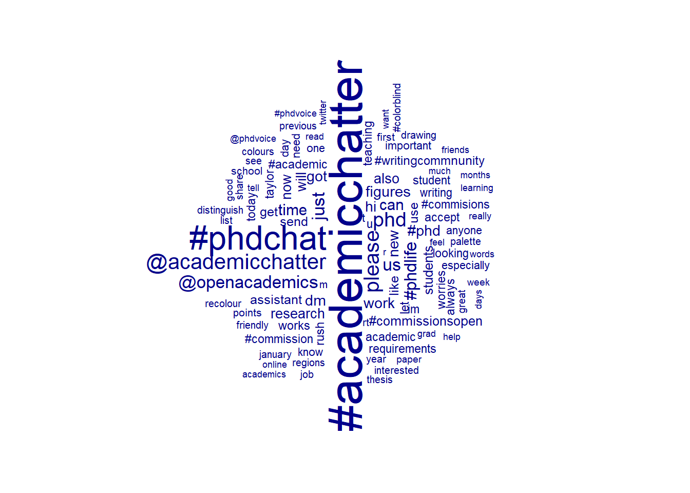
26.4 Dictionaries
Finally, we’ll look at dictionaries.
In quanteda, we can build dictionaries that allow us to count the frequency of dictionary words in different documents. Below, we build a dictionary using the dictionary() function for word related to corruption/illicit activities and words related to a politician.
Learn more about dictionaries here.
my_dict <- dictionary(list(phd = c("#phdadvice", "phd", "#phdlife", "#phdchat"),
                          research = c("thesis", "paper", "papers", "figures", "article", "articles")))
#dictionary creates two dictionaries

tw_dictionary <- dfm_lookup(tw_dfm, dictionary = my_dict)
# we can then add this dictionary to the dictionary argument of dfm

head(tw_dictionary)
## Document-feature matrix of: 6 documents, 2 features (75.00% sparse) and 3 docvars.
## features
## docs phd research
## 1350134035012587520 0 2
## 1350134027496415232 0 1
## 1350133988820742144 0 0
## 1350133880104366080 0 0
## 1350133743344730112 0 2
## 1350133571265171456 0 0The tw_dictionary dfm now produces a count of the number of times a word from the politician dictionary and the illegal dictionary appear in a given tweet.
26.5 Stemming
The last thing we’ll talk about in this tutorial is stemming. Stemming is the process of removing removing stems (suffixes and prefixes) from a word. This helps us consolidate words like “immigration”, “immigrating”, “immigrant”, and “immigrants” into one stem. With stemming, we can count the frequency of root words (“immigra”).
Below, we stem words in the dfm tw_dfm.
## Document-feature matrix of: 6 documents, 20,055 features (99.92% sparse) and 3 docvars.
##                      features
## docs                  please always use #colorblind friendly palette drawing figures especially colours
##   1350134035012587520      1      1   1           1        1       1       1       2          1       1
##   1350134027496415232      0      0   0           0        0       0       0       0          0       0
##   1350133988820742144      0      0   0           0        0       0       0       0          0       0
##   1350133880104366080      0      0   0           0        0       0       0       0          0       0
##   1350133743344730112      1      1   1           1        1       1       1       2          1       1
##   1350133571265171456      0      0   0           0        0       0       0       0          0       0
## [ reached max_nfeat ... 20,045 more features ]## Document-feature matrix of: 6 documents, 16,136 features (99.90% sparse) and 3 docvars.
## features
## docs pleas alway use #colorblind friend palett draw figur especi colour
## 1350134035012587520 1 1 1 1 1 1 1 2 1 1
## 1350134027496415232 0 0 0 0 0 0 0 0 0 0
## 1350133988820742144 0 0 0 0 0 0 0 0 0 0
## 1350133880104366080 0 0 0 0 0 0 0 0 0 0
## 1350133743344730112 1 1 1 1 1 1 1 2 1 1
## 1350133571265171456 0 0 0 0 0 0 0 0 0 0
## [ reached max_nfeat ... 16,126 more features ]One thing you’ll notice is that the overall number of features gets smaller. this is because words like “supporters”, “supporting”, and “supporter” has been collapsed together with “support” (the stem).
But what happens when you have words like “think”, “thinker”, “thinking”, and “thought”? Unfortunately, “thought” won’t be collapsed into the “think” stem. For this process, we would need a more advanced strategy, called lemmatization. We won’t discuss lemmatizations in this tutorial (or class), but you can learn more about how to lemmatize with quanteada here.
set.seed(100)
textplot_wordcloud(tw_dfm_stem, min_count = 1000, random_order = FALSE,
                   rotation = .25) #needed at least a count of 1000 to appear
26.6 Additional
26.6.1 Additional Reading
One of the nice things about quanteda is the ability for you to use dfm’s and quanteda corpora with other NLP packages.
Learn more about quanteda and topicmodels here: https://tutorials.quanteda.io/machine-learning/topicmodel/
Learn more about quanteda and spaCy (POS tagger) here: https://github.com/quanteda/spacyr/blob/master/README.md
26.6.2 Additional Tutorial
University of Virginia Tutorial: https://data.library.virginia.edu/a-beginners-guide-to-text-analysis-with-quanteda/
Social Media Content and quanteda: http://pablobarbera.com/social-media-upf/code/02-quanteda-intro.html
More on quanteda’s corpus structure: https://www.rdocumentation.org/packages/quanteda/versions/1.2.0/vignettes/design.Rmd