Chapter 10 Data Visualizations
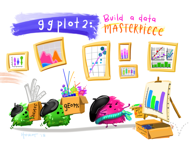
Hello! Today, we’re going to work with ggplot2. This code builds on the code that we have been learning.
Let’s first make sure we set up our code by bringing the tidyverse package into our library. For this class, we will be using data from tidytuesdayR. You can access this data using the tidytuesdayR package (see below).
library(tidyverse)
#install.packages("tidytuesdayR")
#library(tidytuesdayR)
tuesdata <- tidytuesdayR::tt_load('2020-09-15')
##
## Downloading file 1 of 1: `kids.csv`Tidy Tuesday data comes in a tt_data (tidytuesday data) structure, in which there is at least one tibble or data frame. Tibbles are data frames with a few extra bells and whistles (you can learn more about tibbles here). Anything you can do with a data frame, you can do with a tibble.
## spc_tbl_ [23,460 x 6] (S3: spec_tbl_df/tbl_df/tbl/data.frame)
##  $ state           : chr [1:23460] "Alabama" "Alaska" "Arizona" "Arkansas" ...
##  $ variable        : chr [1:23460] "PK12ed" "PK12ed" "PK12ed" "PK12ed" ...
##  $ year            : num [1:23460] 1997 1997 1997 1997 1997 ...
##  $ raw             : num [1:23460] 3271969 1042311 3388165 1960613 28708364 ...
##  $ inf_adj         : num [1:23460] 4665309 1486170 4830986 2795523 40933568 ...
##  $ inf_adj_perchild: num [1:23460] 3.93 7.55 3.71 3.89 4.28 ...
##  - attr(*, "spec")=
##   .. cols(
##   ..   state = col_character(),
##   ..   variable = col_character(),
##   ..   year = col_double(),
##   ..   raw = col_double(),
##   ..   inf_adj = col_double(),
##   ..   inf_adj_perchild = col_double()
##   .. )
## - attr(*, "problems")=<externalptr>##
## addCC CTC edservs edsubs fedEITC fedSSI HCD HeadStartPriv highered lib Medicaid_CHIP
## 1020 1020 1020 1020 1020 1020 1020 1020 1020 1020 1020
## other_health othercashserv parkrec pell PK12ed pubhealth SNAP socsec stateEITC TANFbasic unemp
## 1020 1020 1020 1020 1020 1020 1020 1020 1020 1020 1020
## wcomp
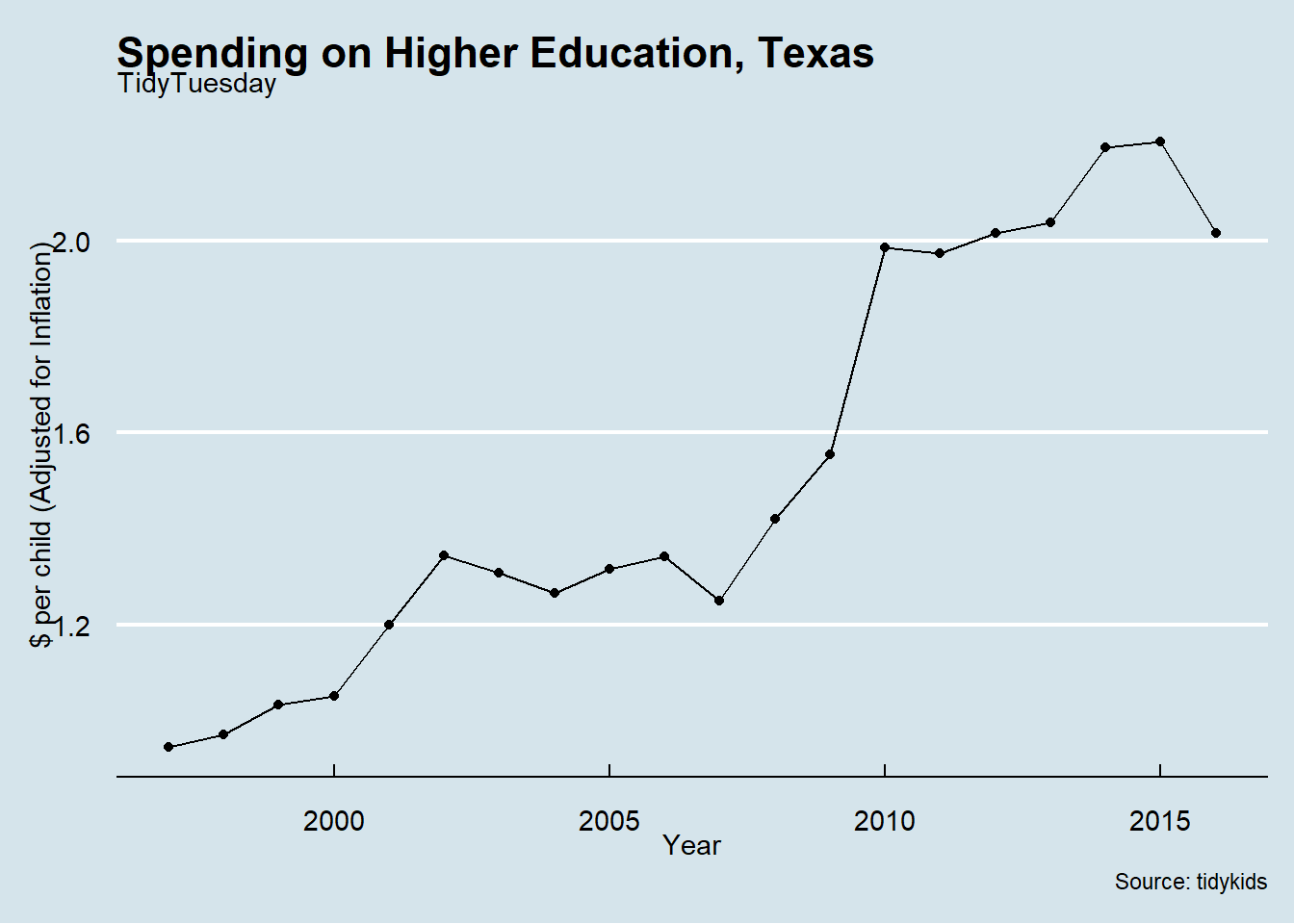
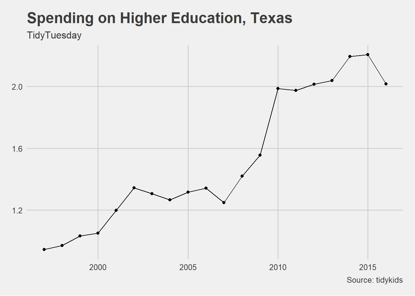
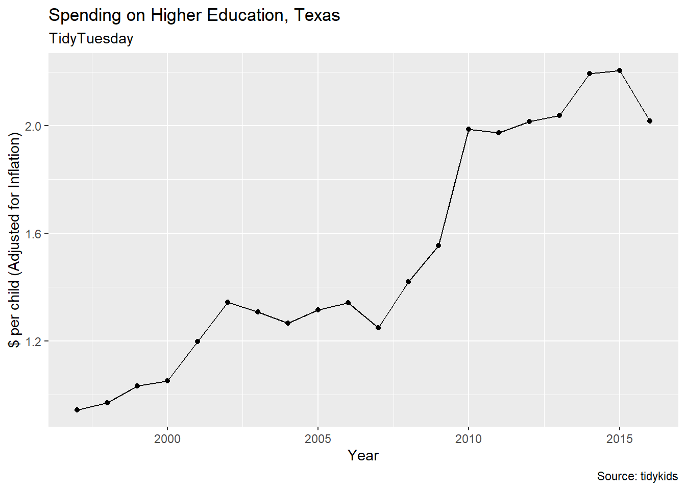
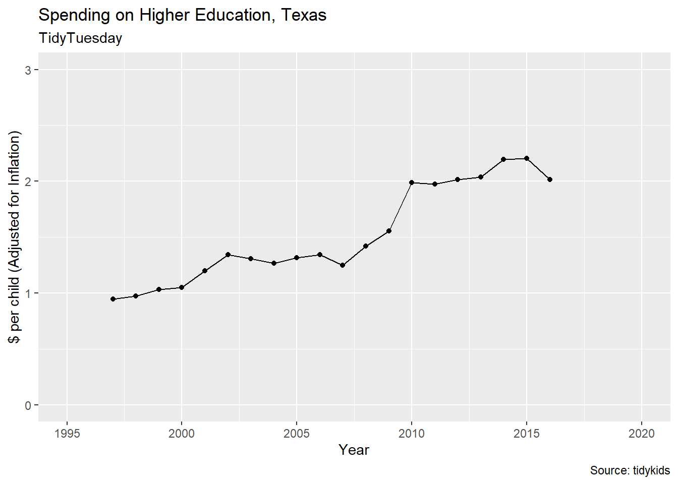
## 1020Let’s replicate the line graph we made in class.
highered_data <- subset(kids_data, variable == "highered")
texas_data <- subset(highered_data, state == "Texas")
#higher_data #you can comment out lines that you are not working on. This is helpful for troubleshooting code
#str(higher_data)
#summary(higher_data)

plot <- ggplot(texas_data, aes(x = year, y = inf_adj_perchild)) + #here, we re-create our graph
  geom_point() +
  geom_line() +
  labs(title = "Spending on Higher Education, Texas",
       subtitle = "TidyTuesday",
       x = "Year", y = "$ per child (Adjusted for Inflation)",
       caption = "Source: tidykids")
plot
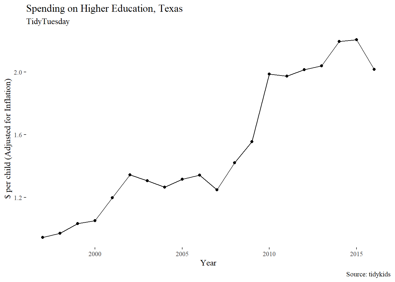
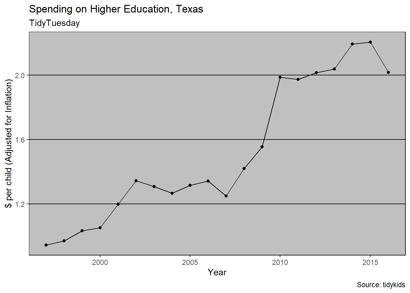
There are a variety of other preset themes you can check out:

 Notice that I can build on a
 ggplot() object with additional + features (these results will not save in the R enviornment until I assign it to the a ggplot object, though).
Because of the popularity of ggplot2, there are a lot of cool packages that build on it, like ggthemes.
10.1 Adding more information
But maybe we want to look at more than one state. Let’s subset our data to do so.
texas_adj_data <- subset(kids_data, variable == "highered") %>%
  subset(grepl("Texas|Oklahoma|Arkansas|New Mexico|Louisiana", state))
In the above chunk, I first look for all rows in which the variable is “highered”. In the next line, I subset rows in which the variable state contains one of the following: Texas, Oklahoma, Arkansas, or New Mexico. The function grepl() is a base R function that returns TRUE if the substring exists in the row (in this case, state) and FALSE if the substring does not exist. In this example, we also use the character operation | (a pipe) as an “or”. Thus, "Texas|Oklahoma|Arkansas|New Mexico|Louisiana" means “Texas OR Oklahoma OR Arkansas OR New Mexico”.
Let’s add a different line for each state. To do this you would use the color aesthetic (aes) in the geom_line() geom. Recall that geoms can can have aes() variable information. This is especially useful for working with a third variable (like when making a stacked bar chart or line plot with multiple lines). Notice that the color aesthetic (meaning that it is in aes) takes a variable, not a color. You can learn how to change these colors here.
ggplot(texas_adj_data, aes(x = year, y = inf_adj_perchild)) +
  geom_point() +
  geom_line(aes(color = state)) +
    labs(title = "Spending on Higher Education, Texas and Bordering States",
       x = "Year", y = "$ per child (Adjusted for Inflation)",
       caption = "Source: tidykids") #you can also create plots without saving them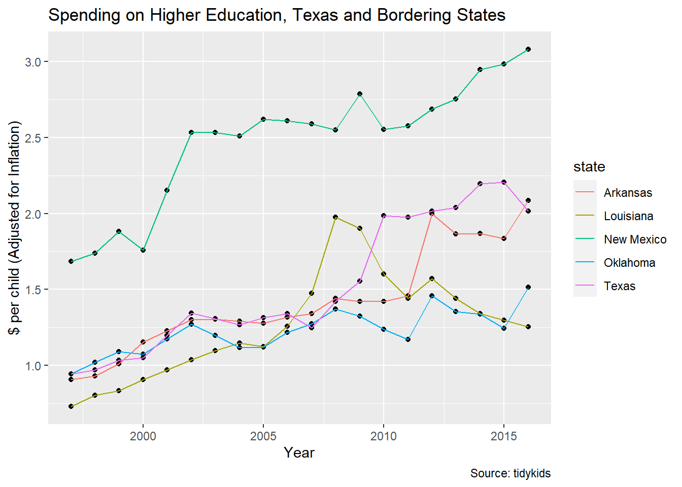
Notice that R changes the color of the line, but not the point? This is because we only included the aesthetic (aes()) to the geom_line geom and not the geom_point geom.
ggplot(texas_adj_data, aes(x = year, y = inf_adj_perchild)) +
  geom_point(aes(color = state)) +
  geom_line(aes(color = state)) +
  labs(title = "Spending on Higher Education, Texas and Bordering States",
       x = "Year", y = "$ per child (Adjusted for Inflation)",
       caption = "Source: tidykids")
We can add other information, like the size (width) of the line:
ggplot(texas_adj_data, aes(x = year, y = inf_adj_perchild)) +
  geom_point(aes(color = state)) +
  geom_line(aes(color = state), size = 2) +
  labs(title = "Spending on Higher Education, Texas and Bordering States",
  x = "Year", y = "$ per child (Adjusted for Inflation)",
  caption = "Source: tidykids")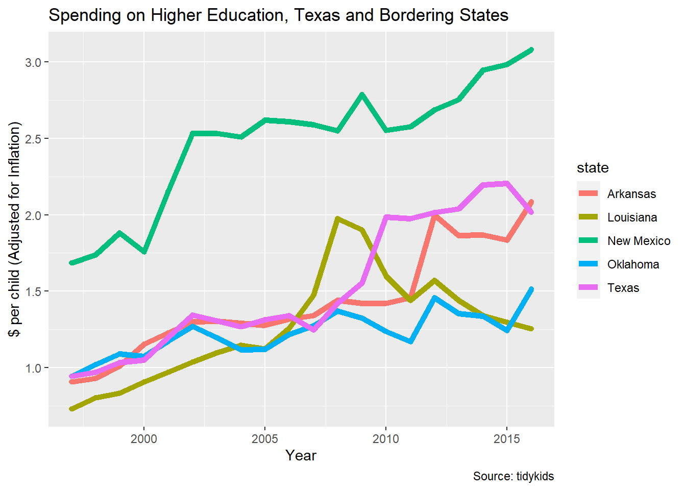
We can change the linetype in the aes to vary line types (like below). This is useful for black and white or greyscale prints.
ggplot(texas_adj_data, aes(x = year, y = inf_adj_perchild, linetype = state)) +
  geom_point() +
  geom_line(size = 1) +
  labs(title = "Spending on Higher Education, Texas",
  x = "Year", y = "$ per child (Adjusted for Inflation)",
  caption = "Source: tidykids")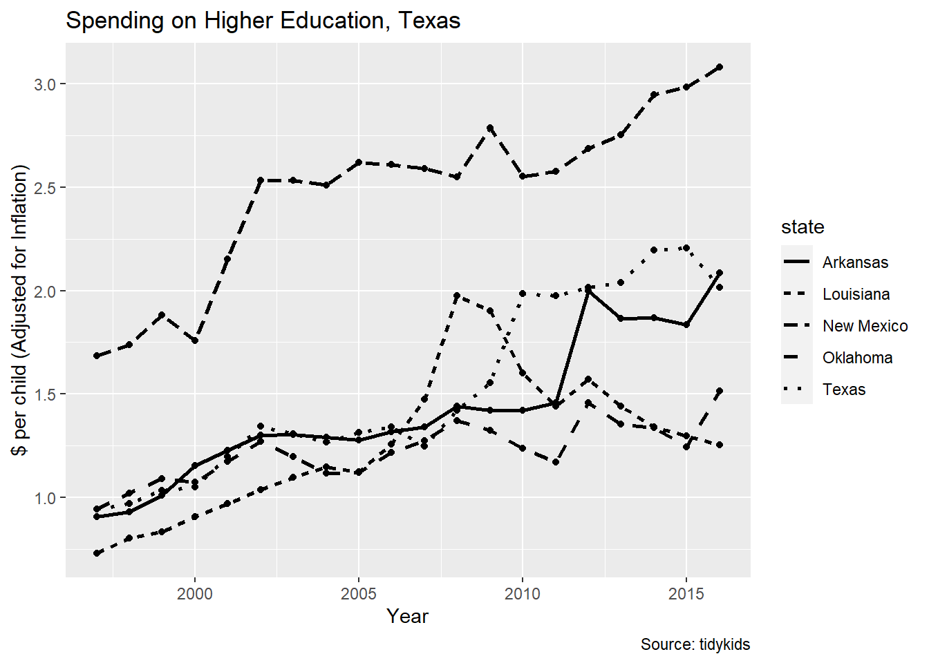
If we wanted to make all the linetypes the same (as opposed to different by another variable), we can put the linetype argument outside of the aes argument (you couldn’t use a variable, but you could choose the linetype for all the variable).
ggplot(texas_adj_data, aes(x = year, y = inf_adj_perchild)) +
  geom_point(aes(color = state)) +
  geom_line(aes(color = state), size = 2, linetype = "dotted") +
  labs(title = "Spending on Higher Education, Texas",
  x = "Year", y = "$ per child (Adjusted for Inflation)",
  caption = "Source: tidykids")
10.2 Facets
Want to plot states in different charts? You can use facet_grid (which you layer on top of the other layers). If added to a ggplot2 variable, you can separate the data by specific variables, and into separate figures (rows displays the figures on top of each other, and cols displays the figures next to one another).
facet_plot <- ggplot(texas_adj_data, aes(x = year, y = inf_adj_perchild)) +
  geom_point() +
  geom_line(size = 1)

facet_plot + facet_grid(rows = vars(state))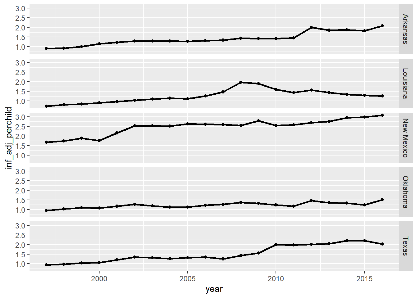
10.3 geom_bar
There are other geoms that you can use to look at different data. For example, let’s use the geom_bar() geom now.
ggplot(data = texas_adj_data, aes(x = year, y = inf_adj_perchild, colour = state)) +
  geom_bar(stat="identity") +
  labs(title = "Spending on Higher Education, Texas",
       x = "Year", y = "$ per child (Adjusted for Inflation)",
       caption = "Source: tidykids")
(Learn more about why we use the
 stat = "identity argument in the geom_bar() geom here.)
Note that the color (or colour) aesthetic doesn’t actually add state information. That is because color refers to the colors of the lines. Intead, what you are probably looking for is fill.
barchart <- ggplot(data = texas_adj_data, aes(x = year, y = inf_adj_perchild, fill = state)) +
  geom_bar(stat="identity") +
  labs(title = "Spending on Higher Education, Texas",
       #subtitle = #did you know you could also put a subtitle here? Try it out!
       x = "Year", y = "$ per child (Adjusted for Inflation)",
       caption = "Source: tidykids")

barchart
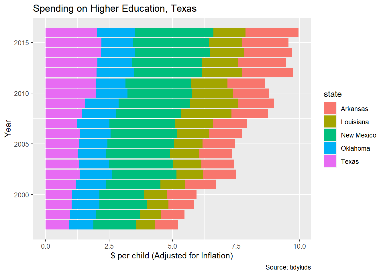 As you can see,
 ggplot defaults to a stacked bar chart. However, you can also separate these out using position_dodge() in the position argument of geom_bar.
ggplot(data = texas_adj_data, aes(x = year, y = inf_adj_perchild, fill = state)) +
  geom_bar(stat="identity", position=position_dodge()) +
  labs(title = "Spending on Higher Education, Texas",
       x = "Year", y = "$ per child (Adjusted for Inflation)",
       caption = "Source: tidykids")
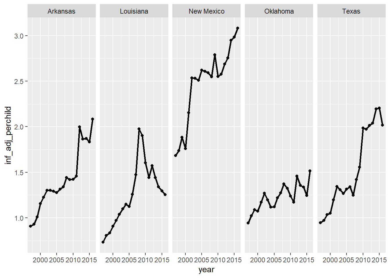
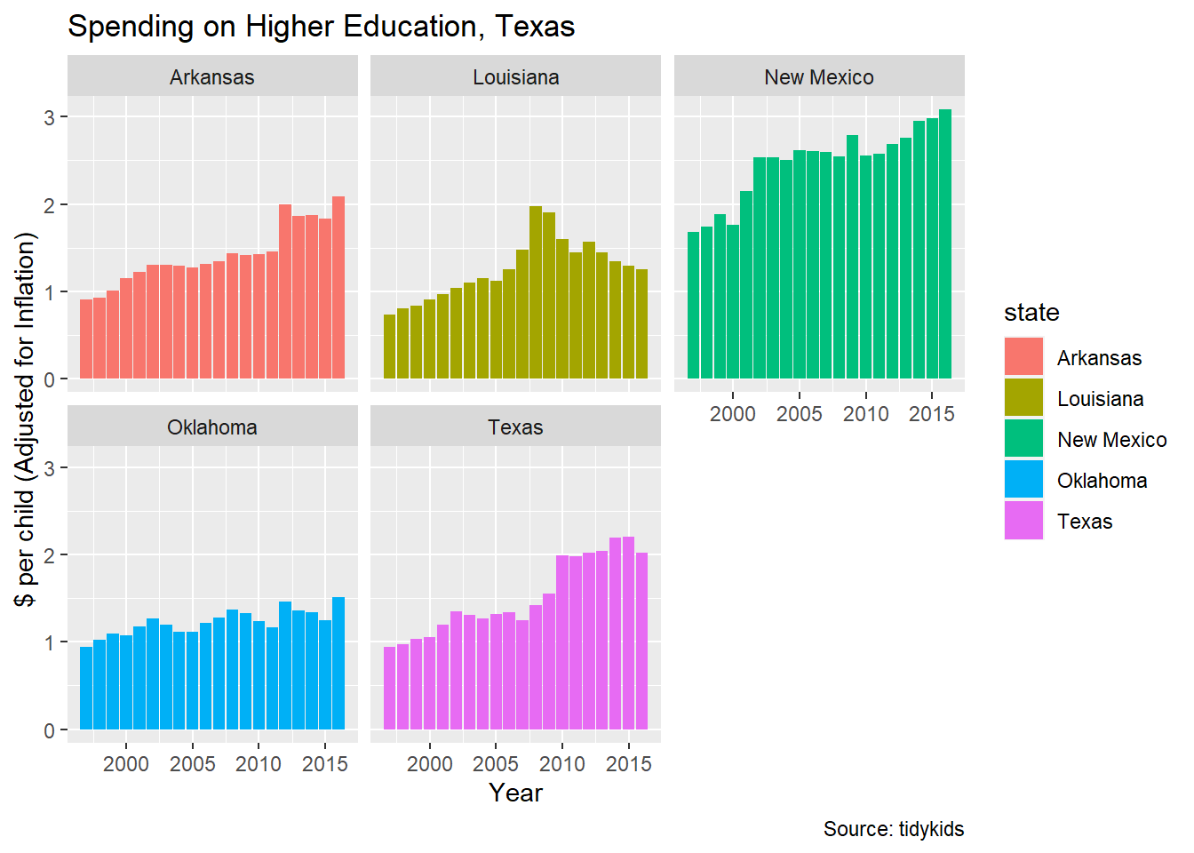
Naturally, you can also use facet_grid, or facet_wrap. (Learn more about the difference here!)

geom_bar() is similar to another geom geom_histogram(), for histograms. Generally geom_bar() is used for frequencies of categories, while geom_histogram() helps you visualize the distribution of a variable. One difference between geom_bar() and geom_histogram() is that geom_histogram() does not take y-variables. Learn more about the difference here.
For more on barplots, check out this guide.
10.4 geom_boxplot
Another geom that may be of interest to you is geom_boxplot(). To use geom_boxplot() one of your variables (x in your aes()) must be a factor
texas_adj_data %>%
mutate(state = as.factor(state)) %>%
ggplot(aes(x = state, y = inf_adj_perchild)) + #notice that you can also pipe in ggplot()
geom_boxplot() + #here is the geom_boxplot() geom
coord_flip() #let's make the boxplots horizontal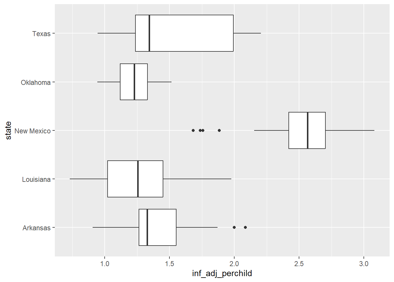 Learn more about boxplots here.
10.5 Themes
We’ve already gone over some of the cool default themes available in ggplot2 (and in other supporting packages), but understanding what can be modified using theme() is very helpful for making your own themes. You can use theme() in combination with default themes to modify them as well.
10.5.1 Margins
For example, to increase the margins around a plot, you would use the plot.margin argument in theme(). We’ll practice using a plot we made earlier (a line graph of yearly spending on Texas higher education).
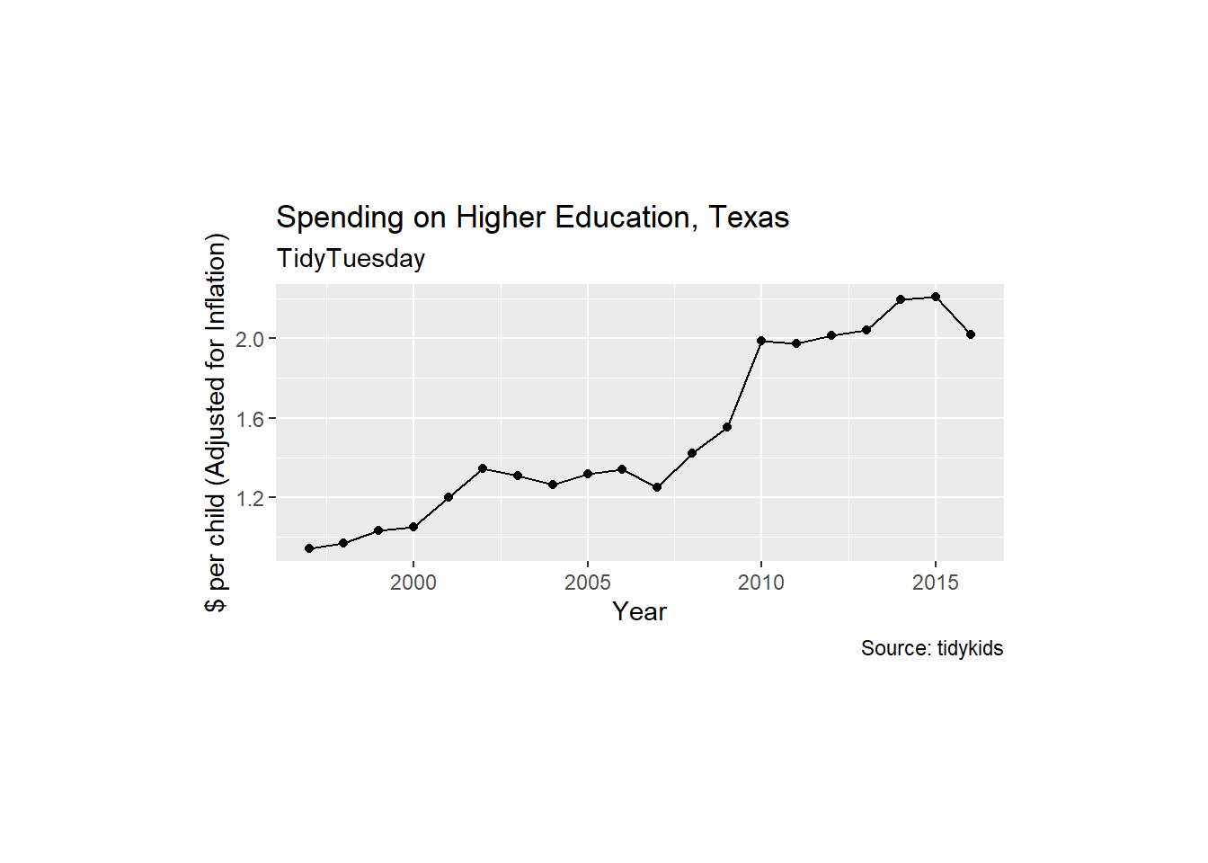
What if you wanted space between the title and the plot? Use the plot.title() argument! This takes an element_text() output (as you can see below).

10.6 Text Size
Using theme(), you can modify a whole variety of things, including the text of the axis, the legend spacing, and even the font of the text!
plot + theme(plot.title = element_text(size = 20, face = "bold"), #you can also change the text facetype
plot.subtitle = element_text(size = 14, color = "red"), #or the color!
axis.title = element_text(size = 14),
axis.text = element_text(size = 12)
) 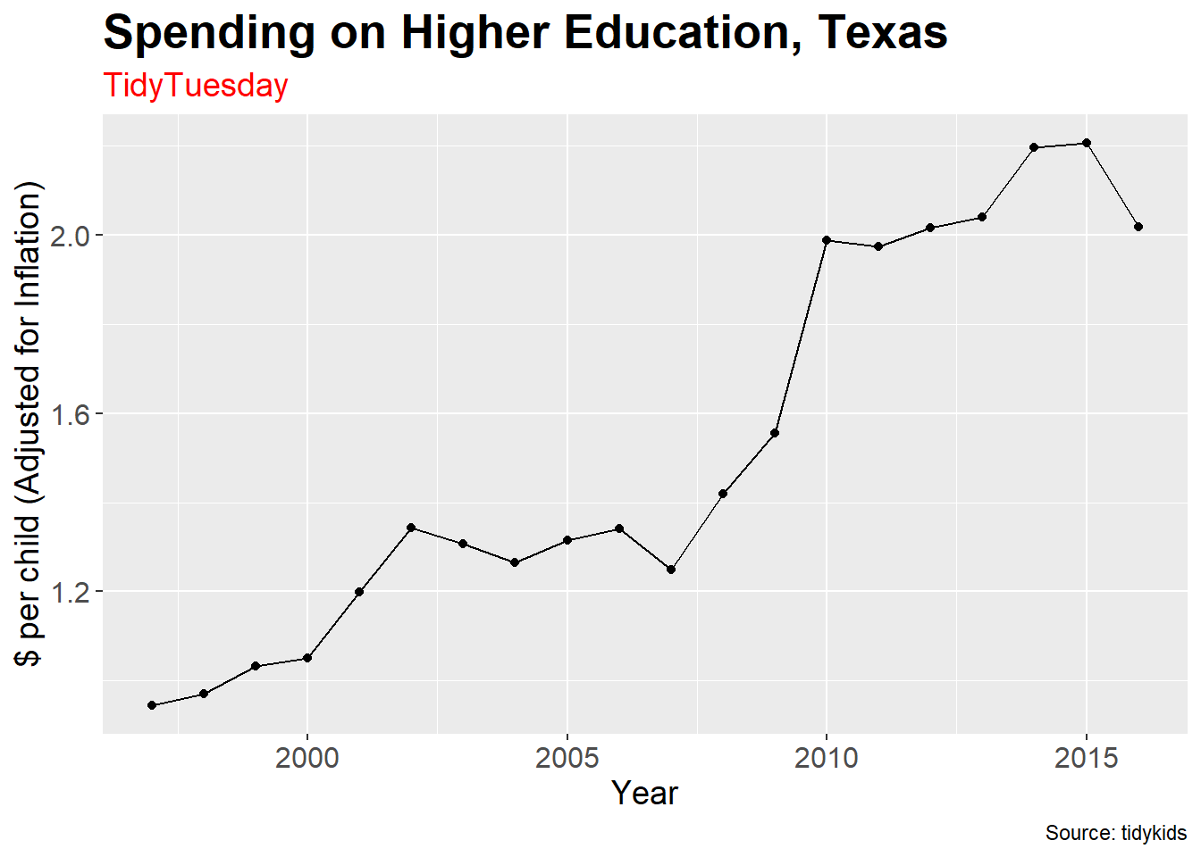 Learn more theme tricks here.
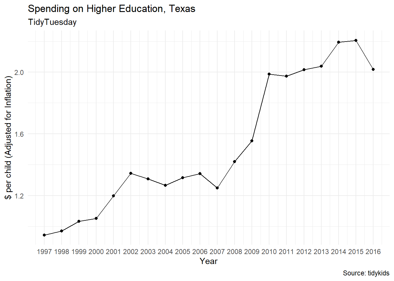
10.7 Axis Scales
ggplot() typically makes assumptions about scale. Sometimes, you may want to change it though (e.g., make them a little larger). There are a couple different ways to do this. The most straightfoward may be xlim() and ylim() (see below)
If you have continuous variables, you can also use scale_x_continuous() and scale_y_continuous(). (These also allow you to modify the names of your x-axis and y-axis, but we’ve already done this through labs()!) For example, if you wanted to add tick marks for every year in our plot, you could do so with the breaks argument in scale_x_continuous().

 There is a parallel for discrete variables, which you can learn about here.
10.8 Saving
To save plots, you can right-click plots that you make in rmarkdowns/r notebooks. Or, you can use the export button in the Plot pane. Or (and this is my preferred strategy), you can save them using ggsave() (learn more here).
## Saving 7 x 5 in image## Saving 7 x 5 in imageIt is important to note that these png figures will be saved in your working directory.
One reason I use ggsave() is that I can save very large figures with higher dpi (dots per inch). This is important because some journals have a minimum dpi for figures (no one wants a fuzzy figure in their journal article).
ggsave("my_other_ggplot.png", plot = plot,
       width = 10, height = 8, units = "in", #the width is 10 inches & the height is 8 inches
       dpi = "print") #look at ?ggsave for more information about these arguments
Note that if you use the same file name for a new figure, R will save over the old figure.
There is no way to show you all the cool things you can do with a short ggplot2 tutorial. If you want to learn how to make various figures in ggplot2, there are many “mega-tutorials” that will show you how. There are also lots and lots of resources on ggplot2, some of which I list here:
- r-statistics.co
- ggplot2 book
- ZevRoss
- ggplot2 cheatsheet
- Visualization masterlist, from r-statistics.co
- sthda
If you would like some material that walks through some of the information I have in this tutorial, check out these links: 1. UC Business Analytics 2. Data Carpentry 3. A good guide comparing base R plots and ggplot 4. Harvard Tutorial, replicating a plot from The Economist
10.9 Bonus Stuff
10.9.1 Interactive plots
Want to make your plot interactive? Use the package plotly! I use plotly often in my blog to make interactive plots, like the one I showed in class. To use plotly, you’ll want to install the plotly package, add it to your library, and then use the ggplotly() function.
#install.packages("plotly")
library(plotly)

interactive_p <- plot + theme_minimal()

ggplotly(interactive_p)
If you want to share the plot, you can save the ggplotly object as an html widget, or you can upload it to a ploty account (which automatically produces a link for your plot). To do the latter, you will need to set up a plotly account (Learn how to do that here).
10.9.2 Animated Plots
Want to make your plots interactive? Use the package gganimate! This one takes a little bit more time to learn because it adds layers to make your plot move. You will also need helper packages like gifski (if you don’t have gifski installed, gganimate will simply return a bunch of frames).
#gganimate_packages <- c("gganimate", "gifski", "transformr")
#install.packages(gganimate_packages) #you will have to restart R before you can use this package
library(transformr)
library(gganimate)
library(gifski)

texas_adj_plot <- ggplot(texas_adj_data, aes(x = year, y = inf_adj_perchild)) +
  geom_line(aes(color = state, x = year), size = 2) +
  theme_minimal() + #use the theme_minimal default
  theme(plot.title = element_text(size = 24, face = "bold"), #change the plot f
        plot.subtitle = element_text(size = 18),
        axis.title = element_text(size = 18), axis.text = element_text(size = 16),
        legend.position = "bottom", #moves the legend to the bottom
        legend.title = element_text(size = 16, face = "bold"),
        legend.text = element_text(size = 16)
        )

texas_adj_plot

texas_adj_plot + transition_reveal(year) #+
  labs(title = "Spending on Higher Education, Texas and Bordering States, Year: {round(frame_along, 0)}",
       subtitle = "Source: tidykids",
       x = "Year", y = "$ per child (Adjusted for Inflation)",
       caption = "Josephine Lukito (for J381M|TidyTuesday)") +
    transition_reveal(along = year, range = NULL)

#%>% gganimate::animate(height = 700, width = 1000) #you will see the plot in viewer() #texas_adj_plot

anim_save("my_first_animated_plot.gif") #Save your plot! Note that this is similar to ggsave()Rendering an animated figure always takes a little bit of time, so it’s important to be patient! If you wanted to pause your animation, instead of looping it, check this stackoverflow thread.
Check out other cool things you can do with gganimate here.