Chapter 6 Data Structures
Hi! Today, we’re talking about data structures and coding in R.
For this tutorial, we will be working with the mtcars dataset in the dataset package, so make sure to add that package to your library. Let’s also add the tidyverse package, a package we will be using a lot in this course.
##                      mpg cyl  disp  hp drat    wt  qsec vs am gear carb
## Mazda RX4           21.0   6 160.0 110 3.90 2.620 16.46  0  1    4    4
## Mazda RX4 Wag       21.0   6 160.0 110 3.90 2.875 17.02  0  1    4    4
## Datsun 710          22.8   4 108.0  93 3.85 2.320 18.61  1  1    4    1
## Hornet 4 Drive      21.4   6 258.0 110 3.08 3.215 19.44  1  0    3    1
## Hornet Sportabout   18.7   8 360.0 175 3.15 3.440 17.02  0  0    3    2
## Valiant             18.1   6 225.0 105 2.76 3.460 20.22  1  0    3    1
## Duster 360          14.3   8 360.0 245 3.21 3.570 15.84  0  0    3    4
## Merc 240D           24.4   4 146.7  62 3.69 3.190 20.00  1  0    4    2
## Merc 230            22.8   4 140.8  95 3.92 3.150 22.90  1  0    4    2
## Merc 280            19.2   6 167.6 123 3.92 3.440 18.30  1  0    4    4
## Merc 280C           17.8   6 167.6 123 3.92 3.440 18.90  1  0    4    4
## Merc 450SE          16.4   8 275.8 180 3.07 4.070 17.40  0  0    3    3
## Merc 450SL          17.3   8 275.8 180 3.07 3.730 17.60  0  0    3    3
## Merc 450SLC         15.2   8 275.8 180 3.07 3.780 18.00  0  0    3    3
## Cadillac Fleetwood  10.4   8 472.0 205 2.93 5.250 17.98  0  0    3    4
## Lincoln Continental 10.4   8 460.0 215 3.00 5.424 17.82  0  0    3    4
## Chrysler Imperial   14.7   8 440.0 230 3.23 5.345 17.42  0  0    3    4
## Fiat 128            32.4   4  78.7  66 4.08 2.200 19.47  1  1    4    1
## Honda Civic         30.4   4  75.7  52 4.93 1.615 18.52  1  1    4    2
## Toyota Corolla      33.9   4  71.1  65 4.22 1.835 19.90  1  1    4    1
## Toyota Corona       21.5   4 120.1  97 3.70 2.465 20.01  1  0    3    1
## Dodge Challenger    15.5   8 318.0 150 2.76 3.520 16.87  0  0    3    2
## AMC Javelin         15.2   8 304.0 150 3.15 3.435 17.30  0  0    3    2
## Camaro Z28          13.3   8 350.0 245 3.73 3.840 15.41  0  0    3    4
## Pontiac Firebird    19.2   8 400.0 175 3.08 3.845 17.05  0  0    3    2
## Fiat X1-9           27.3   4  79.0  66 4.08 1.935 18.90  1  1    4    1
## Porsche 914-2       26.0   4 120.3  91 4.43 2.140 16.70  0  1    5    2
## Lotus Europa        30.4   4  95.1 113 3.77 1.513 16.90  1  1    5    2
## Ford Pantera L      15.8   8 351.0 264 4.22 3.170 14.50  0  1    5    4
## Ferrari Dino        19.7   6 145.0 175 3.62 2.770 15.50  0  1    5    6
## Maserati Bora       15.0   8 301.0 335 3.54 3.570 14.60  0  1    5    8
## Volvo 142E          21.4   4 121.0 109 4.11 2.780 18.60  1  1    4    2
Don’t forget–you want to make sure that the dataset you are working with is in your environment. You can do this by assigning the mtcars dataset to an object using <-
You can also see (but not edit) the dataset using the View() function.
Notice how I used an underscore in the object name? Using lowercased letters and underscores is the most common method for naming objects in R. Learn more about style in Wickham’s style guide here. For more about naming conventions, read this two-page guide.
6.1 Understanding the Data
Now that we have the dataset mtcars saved to an object, let’s learn more about this data. new_file is a dataset with 11 variables (columns) and 32 observations (rows).
We can print out the name of the variables using names(). Try this out yourself!
## [1] "mpg" "cyl" "disp" "hp" "drat" "wt" "qsec" "vs" "am" "gear" "carb"You can save these names in a new object using the <- assignment. If you recall from last week, we used <- to create a new object.
Next, use the str() function to learn more about each variable. (You should be familiar with str() and summary() from last week).
## 'data.frame':    32 obs. of  11 variables:
##  $ mpg : num  21 21 22.8 21.4 18.7 18.1 14.3 24.4 22.8 19.2 ...
##  $ cyl : num  6 6 4 6 8 6 8 4 4 6 ...
##  $ disp: num  160 160 108 258 360 ...
##  $ hp  : num  110 110 93 110 175 105 245 62 95 123 ...
##  $ drat: num  3.9 3.9 3.85 3.08 3.15 2.76 3.21 3.69 3.92 3.92 ...
##  $ wt  : num  2.62 2.88 2.32 3.21 3.44 ...
##  $ qsec: num  16.5 17 18.6 19.4 17 ...
##  $ vs  : num  0 0 1 1 0 1 0 1 1 1 ...
##  $ am  : num  1 1 1 0 0 0 0 0 0 0 ...
##  $ gear: num  4 4 4 3 3 3 3 4 4 4 ...
##  $ carb: num  4 4 1 1 2 1 4 2 2 4 ...
As you can see, the object new_file is a data.frame type (we’ll return to this later). There are 11 variables in this dataset. In this situation, all the variables are numeric (num). But, let’s talk about some of the other data types we are likely to see.
6.2 Data Types
“Numerics” (num) and “integers” (int) are both numbers. You can consider integers to be a special type of numeric. Integers only contain whole numbers, while “Numerics” are more like “floats” or “doubles.” You can learn more about them here.
“Characters” are letters (and numbers and symbols) that collectively constitute a string (i.e., a string of letters). Character objects/vectors/variables are the backbone of Natural Language Processing. You can tell when a value is a character type because it will be in double quotation marks (6 is a number but "6" is a string).
“Logical” objects are binaries: TRUE OR FALSE.
“Factor” objects tend to be categorical variables (e.g., race). Factors are actually integers, but they have labels (called levels) that are characters. In other words, each integer is identifiable by its level or label. Most of the variables in this dataset are factors. Berkeley posted a great tutorial on factors. We’ll also talk a lot about factors when we deal with public opinion data!
To figure out what type your object is, you can use summary(), which is a really useful function for getting some descriptive information about your variables. You can also use class(), which is a function specifically to get the class-type of the object. Try these now in the space below!
##       mpg             cyl             disp             hp             drat             wt             qsec             vs               am              gear
##  Min.   :10.40   Min.   :4.000   Min.   : 71.1   Min.   : 52.0   Min.   :2.760   Min.   :1.513   Min.   :14.50   Min.   :0.0000   Min.   :0.0000   Min.   :3.000
##  1st Qu.:15.43   1st Qu.:4.000   1st Qu.:120.8   1st Qu.: 96.5   1st Qu.:3.080   1st Qu.:2.581   1st Qu.:16.89   1st Qu.:0.0000   1st Qu.:0.0000   1st Qu.:3.000
##  Median :19.20   Median :6.000   Median :196.3   Median :123.0   Median :3.695   Median :3.325   Median :17.71   Median :0.0000   Median :0.0000   Median :4.000
##  Mean   :20.09   Mean   :6.188   Mean   :230.7   Mean   :146.7   Mean   :3.597   Mean   :3.217   Mean   :17.85   Mean   :0.4375   Mean   :0.4062   Mean   :3.688
##  3rd Qu.:22.80   3rd Qu.:8.000   3rd Qu.:326.0   3rd Qu.:180.0   3rd Qu.:3.920   3rd Qu.:3.610   3rd Qu.:18.90   3rd Qu.:1.0000   3rd Qu.:1.0000   3rd Qu.:4.000
##  Max.   :33.90   Max.   :8.000   Max.   :472.0   Max.   :335.0   Max.   :4.930   Max.   :5.424   Max.   :22.90   Max.   :1.0000   Max.   :1.0000   Max.   :5.000
##       carb
##  Min.   :1.000
##  1st Qu.:2.000
##  Median :2.000
##  Mean   :2.812
##  3rd Qu.:4.000
## Max. :8.000## [1] "data.frame"As you can see, because all the variables are numeric, summary() will provide information like the mean and median. This is slightly different for other data types.
6.3 Data Coercion
Sometimes, you will use a variable or object that is not the type that you want. For example, you may read in something that’s a number, but R sees as a character, like the number_variable we will now create.
## [1] "character"How do we change this to a numeric? We can do so using the as.numeric() function, a base R function.
number_variable <- as.numeric(number_variable)
#if you don't assign your result to an object, it will not be saved.

class(number_variable)
## [1] "numeric"Notice now that the variable class has changed from character to numeric. The process of changing a variable type this way is called coercion. Learn more about coercion here. For each data type, there is a parallel transformation function. For example, if you wanted to do the opposite of what we just did (turn a number into a character), you can use the as.character() function. If a variable cannot be transformed, it will convert into an NA, which is R’s way of telling you that a variable is missing.
## [1] 4## [1] "4"## [1] 4## Warning: NAs introduced by coercion## [1] NAProducing NAs can be especially problematic if you are transforming characters into numbers, so it’s especially important for you to be careful when you are cleaning data, because you don’t want to accidentally turn a string into an NA by turning it into a numeric.
Try this out yourself. Create a string variable “hello” and turn it into a numeric. What is the output?
Now that you know what strings, numerics, factors, and logical are, let’s talk a little more data structures.
Data structures are ways of organizing values. You’ve already heard me reference one, “data frames”. This is the structure of the new_file variable we created earlier. In R, there are a lot of different data structures (one blog post describes 5 basic structures, 4 of which we will talk about here).
6.4 Data Structures
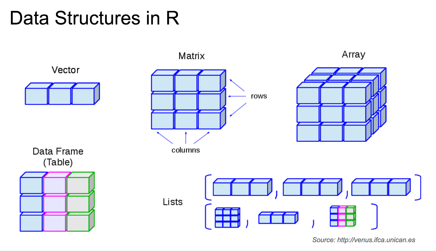
Though objects can be individual things, like a string or a numeric, we are far more likely to work with groups of data types. In this class, we’ll use a couple different types of data structures, including one-dimensional and two-dimensional structures
6.4.1 One Dimensional Strutures
Vectors and Lists
Vectors and lists are the simplest data structures containing more than one value (1-dimensional structures). Of the two, vectors (and more specifically atomic vectors) are the ones you’ll probably use the most in R. Objects in atomic vectors all have the same data type.
You can construct a vector using the c() function, like below:
new_logic_vector <- c(TRUE, TRUE, FALSE, TRUE)
new_string_vector <- c("hello", "world", "hello", "class")
Using class() you can figure out what type of vectors these are. Try that out here!
## [1] "logical"When you create a vector with different types, the c() function will coerce everything into the same data-type. This is an ordered process, as this blog. notes:
There’s a hierarchy of types: the more primitive ones cheerfully and silently convert to those higher up in the food chain. Here’s the order: 1) logical, 2) interger, 3) double, 4) character
That means that if you have a vector of logical and integer values, your logical values will become integer values. If you have a vector of logical, integer, and character values, everything will be coerced into a character value.
## [1] "1" "2" "three" "four" "FALSE"Vectors and lists contain one row of multiple values. When you save a vector, it will appear in the “Values” part of the enviornment. You can isolate items in a vector or list using brackets, [].
## [1] TRUE## [1] "world"Unlike other programming languages (which may start their arrays with 0), vectors and lists in R start with 1.
Though you can use c() to create vectors, the more likely time you’ll encounter them is in more complex data structures. For example, certain columns that you extract from a data frame, data table, tibble, or matrix can be vectors.
You can check whether an object is a vector using the is.vector() function (there are also functions for other data types and structures, like the is.character() function)
## [1] TRUEIt’s worth noting that there are only numeric, character, and logical vectors. Factors are considered numeric vectors with corresponding character values for each level.
Lists are like more generalized vectors. We can create lists using the list()function, but (like vectors), it is more common that you will encouter them in larger datasets. Unlike vectors, lists allow you to hold more complex code. For example, you can have a list with differently sized vectors in them, like in the example we create below:
## [[1]]
## [1] 1 2 3 4 5
##
## [[2]]
## [1] "six"   "seven" "eight"
##
## [[3]]
## [1]  9 10 11 12
##
## [[4]]
## [1] FALSE
##
## [[5]]
## [1] TRUE## [1] "1" "2" "3" "4" "5" "six" "seven" "eight" "9" "10" "11" "12" "FALSE" "TRUE"Note the differences between the new list, new_list, you created versus the new vector, new_vector2. In the former, the list retained the list structure embedded in the data. As a result,new_list[2] contains a character vector with three character objects, “six”, “seven”, and “eight”. In new_vector2, though, you’ll notice that all the objects have been converted into characters, and the internal list structure hasn been removed, or “flattened” so you have 14 observations, rather than a list of 5 vectors of various lengths.
One thing you may have also noticed is the double bracket structure in lists ([[]]). With both vectors and lists, you can use single brackets to extract information from one or more variables
## [1] "1" "2" "3"## [[1]]
## [1] 1 2 3 4 5
##
## [[2]]
## [1] "six" "seven" "eight"
##
## [[3]]
## [1] 9 10 11 12Remember, these results will not save unless you assign it to an object using <-!
Double brackets are unique to lists and can be used to access a single observation or component. One way to think of it is that new_list[1] contains a list ([[1]]), from which you can extract additional information.
## [[1]]
## [1] 1 2 3 4 5## [1] 1 2 3 4 5## [1] 2This is probably one of the harder concepts to understand in R programming. A really good explanation of this bracket structure can be found in our R4DS textbook.
If you would like more reading on vectors and lists:
6.5 Two-Dimensional Structures
Matricies and Data Frames
Most of the data you’ll be working with will be “two-dimensional”: a matrix or (most likely) a data frame. Lots of other data structures, like tibbles and data tables, are built on top of the data frame foundation, but also have additional features.
A UC Riverside tutorial’s description may be helpful: > In essence, the easiest way to think of a data frame is as an Excel worksheet that contains columns of different types of data but are all of equal length rows.
Both matrices and data frames are considered more “complex” data structures because they can have multiple rows and columns (as opposed to lists and vectors, which can have many “rows”, but only one “column”).
You can construct matrices using the matrix() function.
##      [,1] [,2] [,3] [,4] [,5] [,6]
## [1,]    1    3    5    7    9   11
## [2,] 2 4 6 8 10 12## Warning in matrix(1:12, nrow = 3, ncol = 5): data length [12] is not a sub-multiple or multiple of the number of columns [5]## [,1] [,2] [,3] [,4] [,5]
## [1,] 1 4 7 10 1
## [2,] 2 5 8 11 2
## [3,] 3 6 9 12 3In the above examples, I create two matrices containing numbers between 1 and 12. In the first matrix, this is a 2x6 matrix (2 rows, 6 columns). The second matrix is a 3x5. Because there are only 12 numbers, though, the last column is populated with repeated numbers (1 to 3).
You’ll notice that a matrix is populated by row, and then by column.
If you wanted to extract one value from a matrix, you need to know it’s row and column number. You include these numbers in single brackets, [], with a comma in between. This is called subscripting.
new_matrix <- matrix(1:12, ncol = 6, nrow = 2)
new_matrix[2,5] #row number first, column number second
## [1] 10If you subscript just the row or column, you will get all information for that row or column.
## Warning in matrix(1:80, nrow = 20, ncol = 5): data length differs from size of matrix: [80 != 20 x 5]## [,1] [,2] [,3] [,4] [,5]
## [1,] 1 21 41 61 1
## [2,] 2 22 42 62 2
## [3,] 3 23 43 63 3
## [4,] 4 24 44 64 4
## [5,] 5 25 45 65 5
## [6,] 6 26 46 66 6
## [7,] 7 27 47 67 7
## [8,] 8 28 48 68 8
## [9,] 9 29 49 69 9
## [10,] 10 30 50 70 10
## [11,] 11 31 51 71 11
## [12,] 12 32 52 72 12
## [13,] 13 33 53 73 13
## [14,] 14 34 54 74 14
## [15,] 15 35 55 75 15
## [16,] 16 36 56 76 16
## [17,] 17 37 57 77 17
## [18,] 18 38 58 78 18
## [19,] 19 39 59 79 19
## [20,] 20 40 60 80 20## [1] 15 35 55 75 15## [1] 41 42 43 44 45 46 47 48 49 50 51 52 53 54 55 56 57 58 59 60## [1] 55Notice that if I wanted to get all the rows for the 3th variable (the fourth line in the above code chunk), I would leave the first number (the row number) blank.
One cool thing about matrices is the ability to perform matrix algebra (which is essential for many statistical tests and models, including multiple regressions). For example, we can transpose (pivot) a matrix using t().
##       [,1] [,2] [,3] [,4] [,5]
##  [1,]    1   21   41   61    1
##  [2,]    2   22   42   62    2
##  [3,]    3   23   43   63    3
##  [4,]    4   24   44   64    4
##  [5,]    5   25   45   65    5
##  [6,]    6   26   46   66    6
##  [7,]    7   27   47   67    7
##  [8,]    8   28   48   68    8
##  [9,]    9   29   49   69    9
## [10,]   10   30   50   70   10
## [11,]   11   31   51   71   11
## [12,]   12   32   52   72   12
## [13,]   13   33   53   73   13
## [14,]   14   34   54   74   14
## [15,]   15   35   55   75   15
## [16,]   16   36   56   76   16
## [17,]   17   37   57   77   17
## [18,]   18   38   58   78   18
## [19,]   19   39   59   79   19
## [20,] 20 40 60 80 20## [,1] [,2] [,3] [,4] [,5] [,6] [,7] [,8] [,9] [,10] [,11] [,12] [,13] [,14] [,15] [,16] [,17] [,18] [,19] [,20]
## [1,] 1 2 3 4 5 6 7 8 9 10 11 12 13 14 15 16 17 18 19 20
## [2,] 21 22 23 24 25 26 27 28 29 30 31 32 33 34 35 36 37 38 39 40
## [3,] 41 42 43 44 45 46 47 48 49 50 51 52 53 54 55 56 57 58 59 60
## [4,] 61 62 63 64 65 66 67 68 69 70 71 72 73 74 75 76 77 78 79 80
## [5,] 1 2 3 4 5 6 7 8 9 10 11 12 13 14 15 16 17 18 19 20Data frames are like fancier matrices with list/vector properties. Unlike a matrix, which requires every value to be the same type (like a vector), columns in a data frame can be different values. This is especially useful in the event that you have a dataset–like social media data–where some variables are numbers (number of followers), some are strings (usernames), and some are logicals (verified account).
The new_file object is a data frame (as we saw from the str() function). Like a matrix, you can also use brackets to pull out relevant information.
## [1] 4Another very important thing you can do with data frames is pull out individual columns using the $. For example, if you wanted to see the mpg column of new_file, run the following line:
##  [1] 21.0 21.0 22.8 21.4 18.7 18.1 14.3 24.4 22.8 19.2 17.8 16.4 17.3 15.2 10.4 10.4 14.7 32.4 30.4 33.9 21.5 15.5 15.2 13.3 19.2 27.3 26.0 30.4 15.8 19.7 15.0
## [32] 21.4
You can also look at the first 6 observations of this variable using head(). Let’s try this below!
## [1] 21.0 21.0 22.8 21.4 18.7 18.1You can combine this with brackets to identify the n’th row of an observation.
## [1] 6And, you can run functions on individual columns in a data frame, like the as.character() coercion function we learned about previously.
new_file$cyl_string <- as.character(new_file$cyl)
#you can save information to a new column using the <- assignment

new_file$cyl_string[10]
## [1] "6"And, if you run str() on just a specific column of a data frame, R will return the type of variable the column is.
## num [1:32] 6 6 4 6 8 6 8 4 4 6 ...What happens when you use class()? See for yourself:
## [1] "numeric"If you save the columns as a totally new object, you will notice that it is saved as a vector. In other words, each column in a data frame is a vector.
## [1] TRUEYou can play with the is.vector() or is.data.frame() functions to see what R produces:
## [1] TRUE## [1] TRUE## [1] FALSE## [1] FALSE## [1] FALSE## [1] TRUEOne thing you may notice is that new_file$cyl has a finite number of options (4, 6, or 8 cylinders).
## [1] 6 6 4 6 8 6We may want to treat it as a categorical variable (i.e., a factor) rather than keeping it as a numeric. Using one of the coercion functions we learned about above, let us try changing this variable into a factor:
##  [1] 6 6 4 6 8 6 8 4 4 6 6 8 8 8 8 8 8 4 4 4 4 8 8 8 8 4 4 4 8 6 8 4
## Levels: 4 6 8
This will return the output of the function, but it won’t save the results! To save this, you will want to use the <- assignment we have been using this whole time. Try these three sightly different ways of saving variables:
new_file$cyl <- as.factor(new_file$cyl) #saves the results of this coercion to the original variable name
new_file$cyl2 <- as.factor(new_file$cyl) #saves the results in a new column in the data frame
cyl2 <- as.factor(new_file$cyl) #saves the result in a totally new object
Notice that when we turn this numeric into a factor, it will have three “levels. Levels refer to the number of options that the categorical variable could be. For example, if your gender variable includes four options, man, woman, trans/non-binary, no response, you would have 4 levels.
## Factor w/ 3 levels "4","6","8": 2 2 1 2 3 2 3 1 1 2 ...Notice that when the column is a factor, R will also indicate the levels of that factor (this is not displayed for numeric).
If you would like more reading on matrices and data frames: