Chapter 19 Logistic Regression
Hello! Today, we’ll be discussing what logistic regressions are and how we can use this model for machine learning. Let us begin by loading some packages and importing our survey data (the Pew survey we have used previously)
library(tidyverse)
library(broom)
library(datasets)
library(gglm)

survey_data <- read_csv("data/pew_AmTrendsPanel_110_2022_revised.csv")
For the purposes of this tutorial, we are going to focus on the participants who were Democrats or Republicans. This means we will lose some data (e.g., independents, other parties).
If you are interested in advanced solutions for imputing or filling missing data, one package I have come across recently is mice (check out the documentation here and this slightly advanced tutorial here).
For other options to deal with missing data, I encourage you to check out Selva Prabakaran’s tutorial.
What does this data frame look like?
## # A tibble: 6 x 10
##    ...1 perceived_party_difference gun_bill_approval personal_fin party abortion_opinion   age education     income voter
##   <dbl>                      <dbl>             <dbl>        <dbl> <chr>            <dbl> <dbl> <chr>          <dbl> <dbl>
## 1     1                          1                 5            2 rep                  1     4 Some college       3     1
## 2     2                          1                 2            2 rep                  1     4 College Grad+      9     1
## 3     3                          1                 2            3 rep                  1     3 Some college       9     1
## 4     4                          3                 4            4 rep                  1     3 Some college       6     1
## 5     5                          2                 3            2 rep                  1     1 College Grad+      9     1
## 6     8                          1                 2            1 dem                  4     4 Some college       3     1
Huzzah!
Let’s also make sure to clean up the voter variable, which we haven’t done yet
##
##    1    2    3   99
## 2918 126 239 5logistic_data['voter'][logistic_data['voter'] == 1] <- 1
logistic_data['voter'][logistic_data['voter'] == 2] <- 1
logistic_data['voter'][logistic_data['voter'] == 3] <- 0
logistic_data['voter'][logistic_data['voter'] == 99] <- 0
table(logistic_data$voter)##
## 0 1
## 244 3044This data frame (logistic_data) has one label that we will want the computer to model (voter). To do this, we will use three features (i.e., variables: party, education, income, and abortion_opinion) Features are an essential concept in machine learning. Simply put, a feature is one of the variables you put into a machine learning algorithm (you may recognize the term “feature” from quanteda::dfm, which stands for “document-feature matrix”). Machine learning discourse often focuses on “features” (the input) and “labels” (the output), so it’s worth becoming familiar with the language.
Let us now proceed with our logistic regression.
19.1 Logistic Regression
A logistic regression is a useful model when your dependent variable is a bivariate, meaning that there are two values (e.g., “do you intend to vote or not? Do you have COVID-19 or not?”).For this tutorial, we will be using logistic regressions to create a model that will help us estimate whether a person will vote. We can use glm() to create these models. But, rather than using the Gaussian or normal distribution, we will use the binomial distribution by changing the family argument.
19.1.1 Creating Models
v_logit <- glm(voter ~ party + abortion_opinion + education + income, data = logistic_data, family = "binomial")
summary(v_logit)
##
## Call:
## glm(formula = voter ~ party + abortion_opinion + education +
## income, family = "binomial", data = logistic_data)
##
## Deviance Residuals:
## Min 1Q Median 3Q Max
## -2.7113 0.3657 0.3900 0.4225 0.5272
##
## Coefficients:
## Estimate Std. Error z value Pr(>|z|)
## (Intercept) 2.449982 0.125029 19.595 <0.0000000000000002 ***
## partyrep -0.290752 0.134922 -2.155 0.0312 *
## abortion_opinion -0.002694 0.008758 -0.308 0.7583
## educationHS grad or less 0.440193 0.174256 2.526 0.0115 *
## educationSome college 0.129491 0.156287 0.829 0.4074
## income 0.010666 0.005392 1.978 0.0479 *
## ---
## Signif. codes: 0 '***' 0.001 '**' 0.01 '*' 0.05 '.' 0.1 ' ' 1
##
## (Dispersion parameter for binomial family taken to be 1)
##
## Null deviance: 1738.7 on 3287 degrees of freedom
## Residual deviance: 1724.2 on 3282 degrees of freedom
## AIC: 1736.2
##
## Number of Fisher Scoring iterations: 6## Analysis of Deviance Table
##
## Model: binomial, link: logit
##
## Response: voter
##
## Terms added sequentially (first to last)
##
##
## Df Deviance Resid. Df Resid. Dev Pr(>Chi)
## NULL 3287 1738.7
## party 1 3.1499 3286 1735.5 0.07593 .
## abortion_opinion 1 0.0169 3285 1735.5 0.89651
## education 2 6.0291 3283 1729.5 0.04907 *
## income 1 5.2841 3282 1724.2 0.02152 *
## ---
## Signif. codes: 0 '***' 0.001 '**' 0.01 '*' 0.05 '.' 0.1 ' ' 1We can get the output of this logistic regression in one of two ways. The first is to use summary(), as we traditionally have. If we are interested in the cumulative statistical significance of a categorical variable, it may also be useful to use anova().
19.1.2 Model Evaluation
When it comes to logistic regressions, R-squares are not appropriate because the output of a logistic regression is a proportion (likelihood of one of the binaries). However, there are other fit statistics that can help you evaluate how good your logit regression model is.
One particularly useful tool for comparing models is, in fact, the anova() function! Let’s try this now by making a logistic model for likelihood of voting for Trump, but without the party variable.
v_logit_nopty <- glm(voter ~ abortion_opinion + education + income, data = logistic_data, family = "binomial")
#summary(v_logit_nopty)

anova(v_logit_nopty, v_logit) #%>% tidy()
## Analysis of Deviance Table
##
## Model 1: voter ~ abortion_opinion + education + income
## Model 2: voter ~ party + abortion_opinion + education + income
## Resid. Df Resid. Dev Df Deviance
## 1 3283 1728.8
## 2 3282 1724.2 1 4.6394We can also use other diagnostics, like the AIC ( Akaike information criterion) and BIC (Bayesian information criterion), which are both tools for choosing optimal models. You can learn more about model selection tools (or “criteria”) here.
Interpreting AIC and BIC results is easy: the smaller the number, the better the fit. Therefore, when comparing two models, you want to choose the one that is smaller.
## [1] 1736.17## [1] 1738.81## [1] 1772.759## [1] 1769.3Using both the AIC and the BIC, we can see conflicting information: the AIC says v_logit is a better model, whereas the BIC suggests that v_logit_nopty is a better model. This can happen when the models are not too different from one another. To understand this, it is worth getting a better sense of how these criteria select the “best” model. In general, AIC will prefer larger models (models with more variables) because BIC penalizes overly complex models with many parameters that do not provide much information. As mention in this Stack Exchange thread, some folks prefer to use the BIC when trying to select an optimal lag for a time series model. But it is good practice to include the results of both the AIC and BIC for transparency (as a note, this information is often provided in the appendix of a paper, as opposed to the main text).
Want to learn more about using anova() to compare regression models? YaRrr has a great tutorial on that.
19.2 Logistic Regression for ML
But how do we use logistic regression for machine learning? To do this, we have to check the quality of the model that we have created.
To use this logistic regression model for basic machine learning, we will use the popular caret package. caret stands for Classification And REgression Training, and it is extremely popular for programmers using R for machine learning. We’ll be using caret more when we get to the supervised machine learning class, so if you want to get a head start on this content, check out this (long) tutorial by caret author and Rstudio software engineer Max Kuhn. He also has a shorter vignette on caret, which you can find here.
#install.packages("caret")
#caret is a pretty big package with lots of dependencies, so it may take some time to load
library(caret)
19.2.1 Training & Test Sets
Currently, we have one dataset with labels (in our case, “labels” means two variables: a variable for whether someone voted for Biden or not and a variable for whether someone voted for Trump or not). To do supervised machine learning with this dataset, we’ll have to split the data in two. The first part will be used to train a logistic regression model (like we did above). The second part will be used to test the accuracy of the logistic regression model. The second partition allows us to ask: does the logistic regression model we are creating accurately predict our variables of interest?
In caret, there is a useful function called createDataPartition(), which will create an index you can use to split your data. You can also designate the proportion using the p argument in createDataPartition(). A common rule of thumb to split data so that 70 or 80% of the data is used for training and 30 or 20% is used for testing. With larger datasets, you can partition your data further, which is useful if you need to train multiple models, as this person said they did.
Another common reason why you would have more than two partitions (“splits”) is when you want to tweak your parameters as you model. When doing this, it is useful to build a “validation set” by splitting your training set into a training partition (the part you use to train the original model) and a validation partition, which you can use to fine tune your model. The reason you do not use your test set is because you want this test set to remain “pure”–that is, untouched by the model. Remember, you want the test set to test the quality of the model, so the test set should not be used until you are ready to evaluate the final model.
For now, given our sample size (and time), let’s just split our data into two partitions: a training set (80%) and a test set(20%).
split <- createDataPartition(y = logistic_data$voter, p = 0.8,list = FALSE)
#?createDataPartition #learn more about this function

training_set <- logistic_data[split,] #we will use this data to train the model
test_set <- logistic_data[-split,] #we will use this data to test the model
Learn more about data partitions here.
19.2.2 Modeling
Now that we have our partitions, let’s construct our model!
v_logit_trained <- glm(voter ~ abortion_opinion + education + income, data = logistic_data, family = "binomial")
summary(v_logit_trained)
##
## Call:
## glm(formula = voter ~ abortion_opinion + education + income,
## family = "binomial", data = logistic_data)
##
## Deviance Residuals:
## Min 1Q Median 3Q Max
## -2.7342 0.3536 0.4044 0.4151 0.4408
##
## Coefficients:
## Estimate Std. Error z value Pr(>|z|)
## (Intercept) 2.3197537 0.1081188 21.456 <0.0000000000000002 ***
## abortion_opinion -0.0004789 0.0095184 -0.050 0.9599
## educationHS grad or less 0.4029013 0.1732334 2.326 0.0200 *
## educationSome college 0.1147192 0.1560073 0.735 0.4621
## income 0.0100230 0.0053173 1.885 0.0594 .
## ---
## Signif. codes: 0 '***' 0.001 '**' 0.01 '*' 0.05 '.' 0.1 ' ' 1
##
## (Dispersion parameter for binomial family taken to be 1)
##
## Null deviance: 1738.7 on 3287 degrees of freedom
## Residual deviance: 1728.8 on 3283 degrees of freedom
## AIC: 1738.8
##
## Number of Fisher Scoring iterations: 619.2.3 Testing the model
Now that we have our model, we are ready to test it. We’ll do this using the base R function predict(). predict() has two required arguments: a glm model (in our case, t_logit_trained) and the new dataset we want to apply this model to. Because we are using a logistic regression, we will also modify another argument, type. The default to type is scale, which is used to predict numeric dependent variables, so we will change this to type = "response" to make sure we get the right results for a binary dependent variable.
##         1         2         3         4         5         6
## 0.9237294 0.9214799 0.9175475 0.9207516 0.9416337 0.9175475
When reading the head() of this new list of predicted values, you may notice that we do not have a clear “yes” or “no” response. Instead, what we have are proportions: the likelihood that someone is a registered voter. If we want a binary variable, it will be necessary to establish a decision rule. The one we’ll use in this tutorial is: if the model predicts that a person has an over 60% chance of being a registered voter, we will assign that prediction TRUE. If not, we will assign it FALSE.
test_predict_binary <- ifelse(test_predict > 0.6, TRUE, FALSE)
data.frame(test_predict_binary, test_set$voter) %>% head(10)
## test_predict_binary test_set.voter
## 1 TRUE 1
## 2 TRUE 1
## 3 TRUE 1
## 4 TRUE 1
## 5 TRUE 1
## 6 TRUE 1
## 7 TRUE 1
## 8 TRUE 1
## 9 TRUE 1
## 10 TRUE 1As you can already see with these results, our predictions are not completely perfect. With the 9th observation, the participant said they were not a registed voter. However our model predicts that this participant was.
Given this, how can we assess our model to know whether it is really a “good” model? Are there a lot of folks like the participant in row 8, or are they an outlier? Let’s use table() to compare our predicted and true results.
## [1] 0.07914764These results mean that the model is accurate about 92% of the time.
19.3 Bonus: ROC & AUC
Another useful way to evaluate a model is to look at the “ROC curve”. ROC stands for receiver operating characteristic, and ROC curves are common when using a machine learning algorithm to classify binary observations.
A related statistic to this is the AUC, which stands for “Area Under [the ROC] Curve”. When the AUC is high, our classifier is more accurate. AUC scores tend to range from 0.5 (a bad classifier that is no better than random chance) and 1 (a completely accurate classifier).
To construct our ROC curve, we’ll use the package ROCR, which is a great package for visualizing the performance of classifier. Learn more about this package here. For our AUC metric, we’ll use the Metrics package, which contains many functions for evaluating supervised machine learning algorithms. Check out the documentation for this package here.
##
## Attaching package: 'Metrics'
## The following objects are masked from 'package:caret':
##
## precision, recallThe first thing we’ll want to do is create a prediction object using prediction() in the ROCR package. This is the packages’ way of wranging data to use for its other functions. Then, we’ll use performance() to create a performance object, which we can use to plot our ROC. In addition to our prediction object (pr), our performance() function will include two more arguments: measure and x.measure, which are the specific arguments you use to explictly state the evaluation method used. Check out the help page (?performance) for a list of additional performance measures
pr <- ROCR::prediction(test_predict, test_set$voter)

perf <- ROCR::performance(pr,
                          measure = "tpr", #true positive rate
                          x.measure = "fpr") #false positive rate
plot(perf)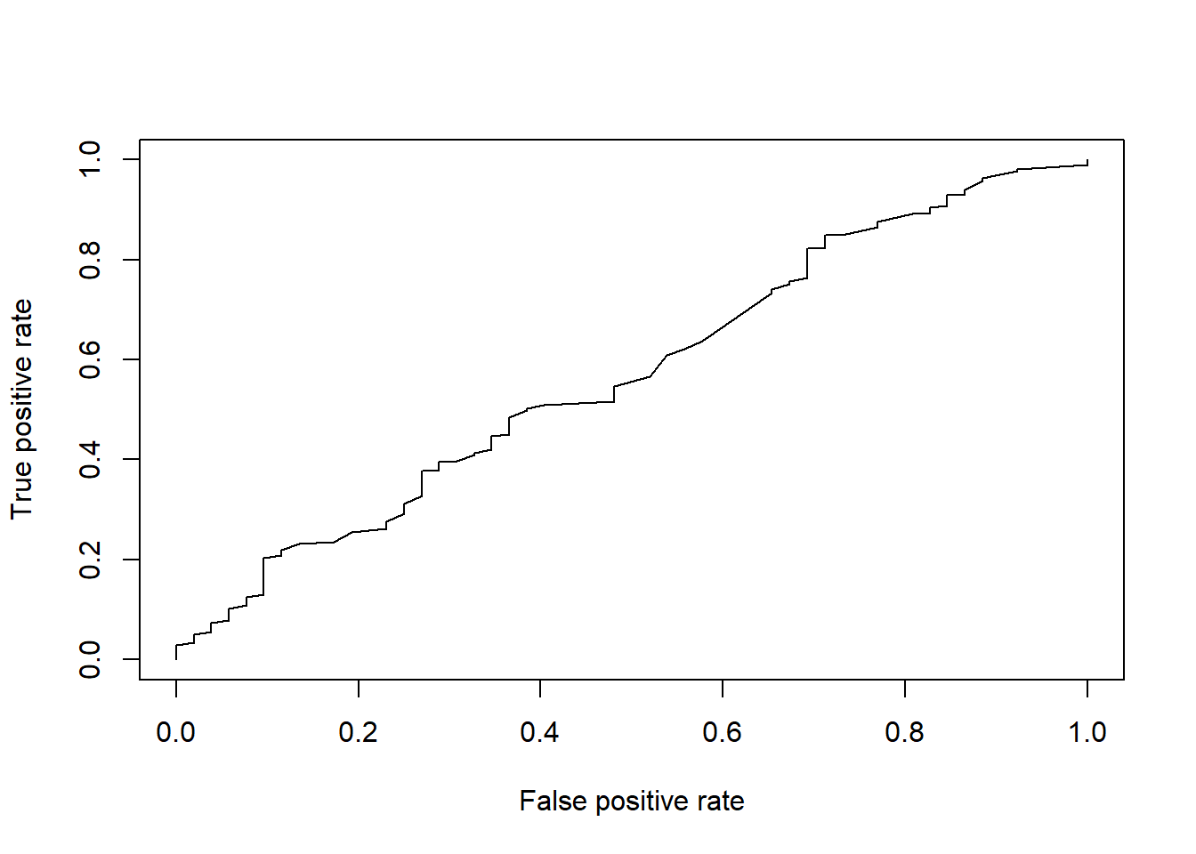
As you see, when we plot() this performance object, the measure argument becomes the y-axis and the x.measure argument is the x-axis. The better the model, the more likely your “curve” will start to appear as a square. A random guess (presumably, 50% accuracy) would look like a vertical diagonal. Thus, your goal as a machine learning programmer is to create a model with a larger “area under the curve.”
To get the actual AUC metric, we can use the auc() function in Metrics, like below.
## [1] 0.5705022That’s an okay AUC.
Want more practice with logit regressions? Check out these tutorials
- Hands on Machine Learning with R textbook
- R Bloggers
- In this tutorial, missing variables are imputed differently
- One Zero Blog
- Towards Data Science
- This site has a couple different tutorials on logistic regression, but I like this one a lot
- If you encounter a paywall, visit the link in incognito/private mode to avoid the paywall
- Hacker Earth
- I’m a fan of how this tutorial discusses the math behind logistic regressions