Chapter 23 Structural Topic Modeling
Hello! Today, we’ll learn about structural topic modeling. For this tutorial, we will use the same data as we did in the LDA topic modeling class. So let’s begin by loading the data!
options(scipen=999)
library(tidyverse)
library(quanteda)
library(tidytext)
library(topicmodels)

library(stm)
tweet_data <- read_csv("data/rtweet_academictwitter_2021.csv") %>%
  select(user_id, status_id, created_at, screen_name, text, is_retweet, favorite_count, retweet_count, verified)
For this analysis, we will again focus on the tweet_data$text column, which contains the tweet message posted by the individual.
23.1 Data Cleaning/Wrangling
This time, in addition to removing URLs, we’re gong to also delete duplicates. The main reason for this is to avoid any one retweet or message “oveweighing” our model. When this step is not done, sometimes you will get a topic model with a topic that is predominantly one tweet or one account. Removing duplicates (which, in the case of Twitter, is typically retweets) can help with this issue.
tweet_data <- tweet_data[!duplicated(tweet_data$text), ]
tweet_data$text <- str_replace_all(tweet_data$text, " ?(f|ht)tp(s?)://(.*)[.][a-z]+", "")
For the wrangling, there are two possible options that you have. The first is to use textProcessor(), the default processor of stm. It is a “wrapper” from tm, which means that it will take the same arguments as tm(). You can use textProcessor() to remove a variety of things, including stopwords, numbers, and punctuation marks (all of these things default to TRUE for removal). There are other things you can remove, so I encourage you to check out the ?textProcessor help page
tweet_processed <- textProcessor(tweet_data$text,
                                 metadata = tweet_data,
                                 lowercase = TRUE,
                                 striphtml = TRUE)
## Building corpus...
## Converting to Lower Case...
## Removing punctuation...
## Removing stopwords...
## Removing numbers...
## Stemming...
## Creating Output...Alternatively, you can also create a quanteda document feature matrix (dfm). Refer back to our Week 8 bonus tutorial on quanteda for more.
23.2 prepDocuments
In addition to this processing step, stm also has one additional step prepDocuments(). This function is used to “clean up” your document term matrix. One reason this step is especially useful is that you can determine an upper or lower threshold for words to include.
Why is this important? As we have discussed, NLP data can be very sparse. When you construct a dfm (or dtm), you may have noticed that your matrix is considered very sparse, like 90% or even 99% scarcity. This is pretty typical of text analysis; after all, you will probably have more words than messages. For this reason, it is sometimes helpful to establish a lower threshold. We state this in prepDocuments() using the lower.thresh argument). In our case, lower.thresh = 20 means that any word appearing in fewer than 20 documents would be automatically excluded from our analysis. This helps make the data less sparse. If you have words that appear too frequently in your corpus (this can be common when you do not include a custom stop word or when the terms you searched by appear in your stm), you can also remove there using the upper.thresh argument.
out <- prepDocuments(tweet_processed$documents, tweet_processed$vocab,
                     tweet_processed$meta, lower.thresh = 20)
## Removing 17986 of 18795 terms (36220 of 98467 tokens) due to frequency
## Removing 16 Documents with No Words
## Your corpus now has 6062 documents, 809 terms and 62247 tokens.23.3 Choosing the K
Like LDA (and other clustering strategie in general), determining a k number of topics can be tricky. In stm, this is done using the searchK() function. This is similar to the LDA k search: it works by building a k model (in this case, we start with 15) and then iteratively compare one model to the next, so k = 15 is compared to k = 16, which is then compared to k = 17 and so on. This results in a somewhat time-consuming process, which is important to keep in mind if you plan to run the next chunk of code.
23.4 Structural Topic Modeling
Let us now proceed with building our structural topic model! One thing you’ll notice about the stm() model is that it takes many arguments. For our analysis, we use the output of the prepDocuments() function (which returns a documents column, a vocab column and a meta column). In addition to this, we also have to state the k number of topics we want (we’ll use 10 here), as well as the init.type (this is similar to the sampling strategy argument in LDA). Finally, there is the prevalence argument, which allows you to specify meta-data variables you are interested in using as covariates. This complicates your model, so you don’t want to throw all your possible meta-data in. But, if you have an especially important meta-data variable, this is one way to account for it.
tweets_stm <- stm(documents = out$documents, vocab = out$vocab,
                       K = 10,
                       prevalence =~ verified,
                       max.em.its = 50,
                       data = out$meta,
                       init.type = "Spectral",
                       seed = 100)
## Beginning Spectral Initialization
## Calculating the gram matrix...
## Finding anchor words...
## ..........
## Recovering initialization...
## ........
## Initialization complete.
## .....................................................................................................
## Completed E-Step (1 seconds).
## Completed M-Step.
## Completing Iteration 1 (approx. per word bound = -6.083)
## .....................................................................................................
## Completed E-Step (1 seconds).
## Completed M-Step.
## Completing Iteration 2 (approx. per word bound = -6.005, relative change = 1.289e-02)
## .....................................................................................................
## Completed E-Step (1 seconds).
## Completed M-Step.
## Completing Iteration 3 (approx. per word bound = -5.960, relative change = 7.362e-03)
## .....................................................................................................
## Completed E-Step (1 seconds).
## Completed M-Step.
## Completing Iteration 4 (approx. per word bound = -5.935, relative change = 4.169e-03)
## .....................................................................................................
## Completed E-Step (1 seconds).
## Completed M-Step.
## Completing Iteration 5 (approx. per word bound = -5.919, relative change = 2.801e-03)
## Topic 1: academictwitt, pleas, share, scienc, can
## Topic 2: write, academ, thank, paper, help
## Topic 3: student, academictwitt, read, book, teach
## Topic 4: academictwitt, academicchatt, openacadem, like, can
## Topic 5: academictwitt, day, join, submit, applic
## Topic 6: academictwitt, academicchatt, phdchat, phd, phdlife
## Topic 7: amp, academictwitt, use, interest, way
## Topic 8: review, academicchatt, love, hard, dont
## Topic 9: academictwitt, just, work, also, got
## Topic 10: academictwitt, feel, academicchatt, one, make
## .....................................................................................................
## Completed E-Step (1 seconds).
## Completed M-Step.
## Completing Iteration 6 (approx. per word bound = -5.908, relative change = 1.856e-03)
## .....................................................................................................
## Completed E-Step (1 seconds).
## Completed M-Step.
## Completing Iteration 7 (approx. per word bound = -5.901, relative change = 1.200e-03)
## .....................................................................................................
## Completed E-Step (1 seconds).
## Completed M-Step.
## Completing Iteration 8 (approx. per word bound = -5.897, relative change = 7.043e-04)
## .....................................................................................................
## Completed E-Step (1 seconds).
## Completed M-Step.
## Completing Iteration 9 (approx. per word bound = -5.894, relative change = 3.602e-04)
## .....................................................................................................
## Completed E-Step (1 seconds).
## Completed M-Step.
## Completing Iteration 10 (approx. per word bound = -5.894, relative change = 1.519e-04)
## Topic 1: academictwitt, pleas, scienc, share, research
## Topic 2: write, academ, paper, thank, help
## Topic 3: academictwitt, student, read, teach, book
## Topic 4: academictwitt, like, year, openacadem, academicchatt
## Topic 5: academictwitt, day, join, today, applic
## Topic 6: academicchatt, academictwitt, phdchat, phd, phdlife
## Topic 7: amp, academictwitt, use, interest, list
## Topic 8: review, love, thought, data, dont
## Topic 9: work, academictwitt, just, first, also
## Topic 10: academictwitt, feel, make, one, anyon
## .....................................................................................................
## Completed E-Step (1 seconds).
## Completed M-Step.
## Completing Iteration 11 (approx. per word bound = -5.893, relative change = 2.904e-05)
## .....................................................................................................
## Completed E-Step (1 seconds).
## Completed M-Step.
## Model Converged23.4.1 Results
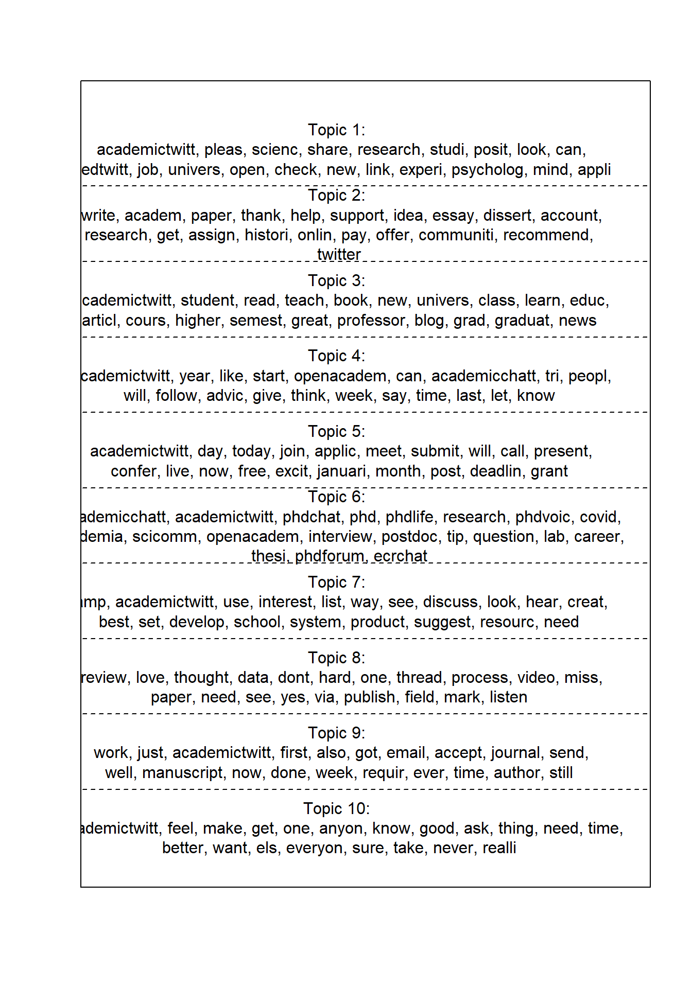
Let’s see what these topics look like!
## Topic 1 Top Words:
##       Highest Prob: academictwitt, pleas, scienc, share, research, studi, posit
##       FREX: pleas, share, posit, scienc, art, link, podcast
##       Lift: psychedel, retweet, militari, studentlif, anthropolog, medit, spiritu
##       Score: retweet, pleas, scienc, share, academictwitt, psychedel, medtwitt
## Topic 2 Top Words:
##       Highest Prob: write, academ, paper, thank, help, support, idea
##       FREX: essay, write, account, assign, idea, thank, pay
##       Lift: studytwtph, studytwt, essay, math, statist, feedback, academicwrit
##       Score: studytwtph, write, essay, academ, thank, paper, assign
## Topic 3 Top Words:
##       Highest Prob: academictwitt, student, read, teach, book, new, univers
##       FREX: read, student, book, blog, higher, cours, teach
##       Lift: malta, maltaunivers, blog, read, introduct, trend, staff
##       Score: maltaunivers, student, read, book, malta, teach, univers
## Topic 4 Top Words:
##       Highest Prob: academictwitt, year, like, start, openacadem, can, academicchatt
##       FREX: give, follow, tri, tweet, year, advic, start
##       Lift: followfriday, noth, weekend, sentenc, minut, tweet, took
##       Score: followfriday, openacadem, academictwitt, like, start, follow, year
## Topic 5 Top Words:
##       Highest Prob: academictwitt, day, today, join, applic, meet, submit
##       FREX: januari, deadlin, meet, abstract, join, submit, grant
##       Lift: march, januari, abstract, deadlin, webinar, regist, februari
##       Score: march, join, januari, deadlin, day, submit, applic
## Topic 6 Top Words:
##       Highest Prob: academicchatt, academictwitt, phdchat, phd, phdlife, research, phdvoic
##       FREX: phdvoic, phdchat, phdlife, phd, phdforum, interview, academicchatt
##       Lift: bbn, researchcultur, phdforum, academicssay, covid-, phdvoic, phdadvic
##       Score: bbn, academicchatt, phdchat, phd, phdlife, academictwitt, phdvoic
## Topic 7 Top Words:
##       Highest Prob: amp, academictwitt, use, interest, list, way, see
##       FREX: amp, system, goal, list, problem, set, use
##       Lift: adeaweb, liar, nyudent, tuftsdent, tuftsunivers, chronicl, white
##       Score: adeaweb, amp, use, chronicl, liar, nyudent, tuftsdent
## Topic 8 Top Words:
##       Highest Prob: review, love, thought, data, dont, hard, one
##       FREX: hard, love, miss, mark, editor, watch, review
##       Lift: imag, coffe, quot, self, econtwitt, matter, editor
##       Score: imag, review, love, hard, econtwitt, mark, thought
## Topic 9 Top Words:
##       Highest Prob: work, just, academictwitt, first, also, got, email
##       FREX: got, just, accept, send, also, requir, email
##       Lift: academicecpnkm, rush, taylor, writingcommnun, commis, worri, send
##       Score: academicecpnkm, just, got, accept, work, send, also
## Topic 10 Top Words:
##       Highest Prob: academictwitt, feel, make, get, one, anyon, know
##       FREX: feel, better, els, ask, make, everyon, sure
##       Lift: seen, els, pretti, better, feel, everyon, refer
##       Score: seen, feel, make, academictwitt, anyon, ask, one
We can show these words differently:
You can also plot the distribution of these topics
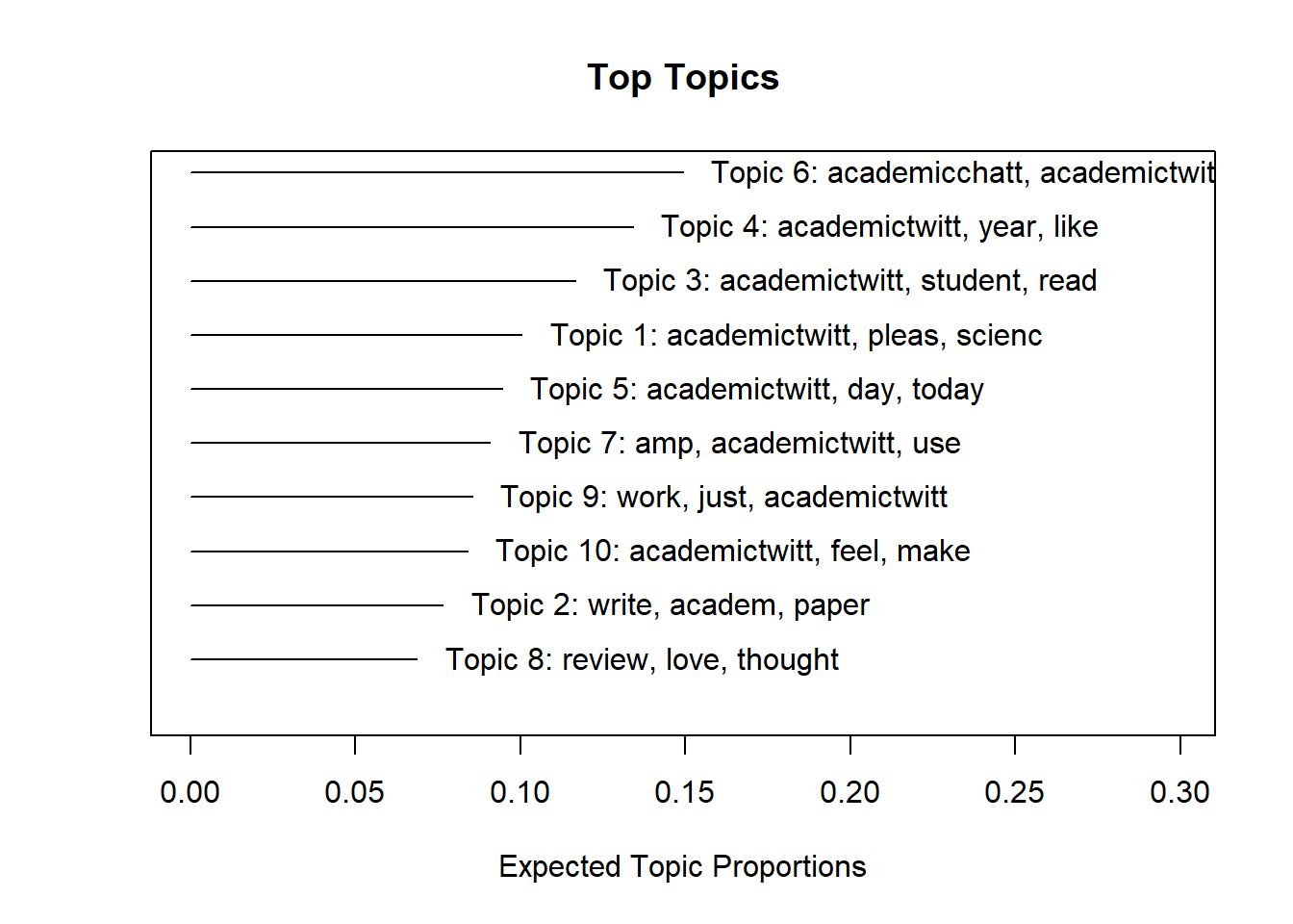
Check out plot.stm() for more information
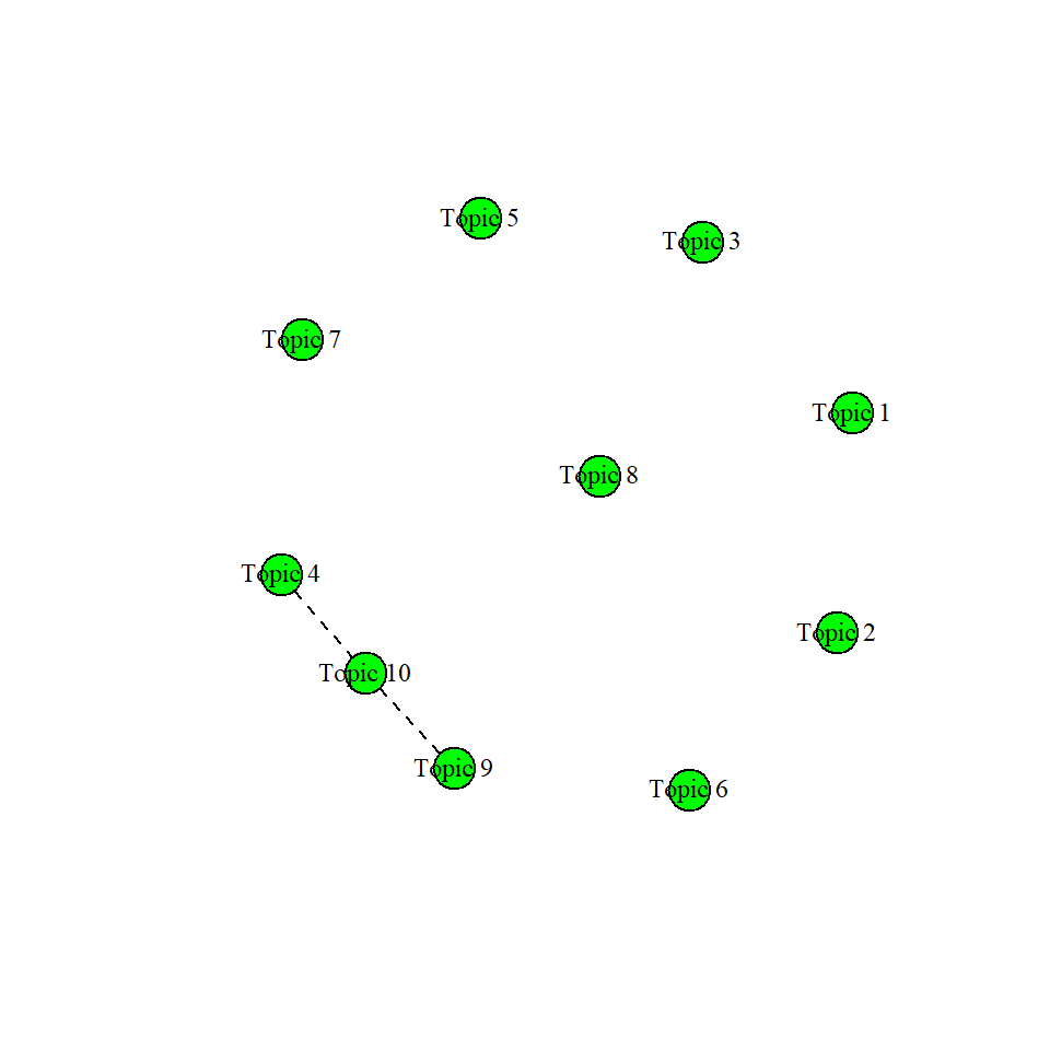
23.4.1.1 Correlations
One thing that distinguished structural topic modeling from LDA topic modeling is the ability to see whether topics are correlated in STM. For this, we will use the topicCorr() function in stm. When we plot the outut of topicCorr(), we get an interesting network diagram of the topics. If there is a line in betweenn those two documents, they are correlated. You can establish a specific cutoff point using the cutoff argument in topiccorr. If you have data that are not quite normal, you may also want to consider changing the default method argument from "simple" to "huge".
23.4.2 Extracting Thetas
In structural topic modeling, gammas (the scores we use to evaluate the proportion that a document belongs to a topic) are called “thetas.” Don’t be confused by the word-change: thetas serve a similar function to gamma scores: they allow you to figure out how to assign a topic to each document.
theta_scores <- tweets_stm$theta %>% as.data.frame()
theta_scores$status_id <- out$meta$status_id #from the "out" processed file
#View(theta_scores)
If you View(theta_scores), you’ll notice that tweets_stm$theta is already structured in a wide format. To isolate the topics with the highest theta for each document (as we did in the LDA tutorial), we will need to convert this to a “long” format.
topics_long <- theta_scores %>%
  pivot_longer(cols = V1:V10,
               names_to = "topic",
              values_to = "theta")
Now that we have our long data, we can proceed with extracting the top thetas…
toptopics <- topics_long %>%
  group_by(status_id) %>%
  slice_max(theta)

colnames(toptopics)[1] <- "status_id"
colnames(toptopics)[2] <- "topics"
toptopics$status_id <- as.numeric(toptopics$status_id)
And plotting our results…
table(toptopics$topics) %>% as.data.frame() %>%
  ggplot(aes(x = Var1, y = Freq)) +
    geom_bar(stat = "identity")
Ta da!
Want more practice with Structural Topic Modeling? Check out these tutorials * https://blogs.uoregon.edu/rclub/2016/04/05/structural-topic-modeling/ * STM Website * Julia Silge’s Tutorial(it also has a great video) * R Bloggers Tutorial