Chapter 22 LDA Topic Modeling
Hello! In this tutorial, we will be learning LDA topic modeling. LDA is a statistical model that is commonly used in topic modeling, a family of unsupervised machine learning strategies that are used for clustering or grouping observations. Topic modeling is a mixed-membership clustering strategy primarily used in natural language processing. This means that each observation (really, each message) is seen as a mix of a group of topics.
For this tutorial, we will be using the Barbenheimer posts (we have used this data before) to learn how to construct an LDA topic modeling. In addition to using tidytext, we will also learn two new packages, topicmodels, which is used for topic modeling algorithms generally, and ldatuning, a package used to determine the optimal number of topics in LDA topic modeling.
Let us now load our packages and import our data.
options(scipen=999)
library(tidyverse)
library(tidytext)
library(janitor)
library(topicmodels)
data_fb <- read_csv("data/crowdtangle_barbenheimer_2023.csv") |>
  clean_names() |>
  select(post_created_date, page_name, message) |>
  mutate(index = 1:16794)
22.1 Data Cleaning/Wrangling
For LDA modeling, we will need the data to be in a document-term matrix (or, in quanteda language, document-feature matrix). To do so, we’ll process our data using the tidytext package we learned in Week 8 (NLP). First, we’ll remove all the URLs using str_replace_all().
Next, we build a custom dictionary of stop words and binds it to an already existing list of stop words in tidytext (stop_words).
final_stop <- data.frame(word = c("said", "u", "0001f6a8", "illvi9k4pg", "https", "t.co", "video", "amp", "2000", "18",
                                  "1", "2", "3", "4", "don", "6", "0001f62d", "im", "fe0f", "30", "barbenheimer", "barbie",
                                  "oppenheimer", "de", "der", "das", "la", "en", "el"),
                         lexicon = "custom") %>%
  rbind(stop_words)
Finally, we prepare our document-term matrix using the cast_dtm() function.
data_dtm <- data_fb %>%
  unnest_tokens(word, text) %>% #tokenize the corpus
  anti_join(final_stop, by = "word") %>% #remove the stop words
  dplyr::count(index, word) %>% #count the number of times a word is used per status_id
  cast_dtm(index, word, n) #creates a document-term matrix

data_dtm
## <<DocumentTermMatrix (documents: 16480, terms: 62534)>>
## Non-/sparse entries: 298281/1030262039
## Sparsity : 100%
## Maximal term length: NA
## Weighting : term frequency (tf)If you need a refresher on document-term matricies, please check out this tutorial. If you’re using quanteda, the “document-term matrix” is synonymous with “document feature matrix”. Learn more here.
22.2 LDA Topic Modeling
Now, let us proceed with our topic modeling. To construct an LDA topic model, we will use the LDA() function in the topicmodels package. For this example, we will categorize our data into 12 topics (k = 12). LDA has two methods for fitting the data, VEM and Gibbs. Choosing a different method will produce slightly different results. Learn more about the difference between VEM and Gibbs here.
Importantly, for you to be able to replicate your results in the future, it is necessary for you to set the seed before proceeding with this analysis. For this tutorial, we will use the see 381. If you do not set a consistent seed, R will randomly generate one for you, which may be problematic for replicating your results.
Another important note: This function takes a while (because your machine learning model is running).
## A LDA_VEM topic model with 8 topics.lda_model contains a wealth of information. The two most important variables in this model are beta and gamma. Let’s look at these in more detail.
22.2.1 beta
beta numbers are assigned to each word in a topic. If a beta score is higher, that word matters more to that topic. In other words, when a message uses that word, it is more likely to be categorized into the affiliated cluster.
We can extract this information using the tidy() function.
Next, we focus on the top 10 words in each topic. To do so, we will use our split-apply-combine pattern by grouping the words by topic (“split”), identifying the top 10 words (“apply”), and then using ungroup() to remove the grouping variable (“combine”).
top_terms <- topics %>%
  group_by(topic) %>% #groups by topic
  top_n(10, beta) %>% #takes the words with the top 10 beta scores
  ungroup() #ungroups the topic
We can also illustrate this data graphically, as you can see below.
top_terms %>%
  ggplot(aes(x = reorder_within(term, beta, topic, sep = "_"),
             y =  beta,
             fill = factor(topic))) +
  geom_bar(stat = 'identity', show.legend = FALSE) +
  facet_wrap(~ topic, scales = "free") +
  coord_flip()
Notably, a lot of our topics are split by language, which is quite interesting!
In this chunk, our aes() has a pretty complicated x-variable. reorder_within() which we use in this line, is a function from tidytext that allows you to reorder a column that you plan to facet later. Here, we want to order the term variable (what becomes the x-variable) by the beta size, but also by topic (since we have a figure for each topic).
The result of doing reorder_within(), however, is that you change the label of the x-variable (which becomes the y-variable when you use coord_flip()). How do we remove that? If we add the ggplot layer scale_x_discrete, we can modify the labels of the x-variable. scale_x_discrete adds a layer to modify the labels of a discrete x-variable; but there are also scale_continuous() ggplot layers you can add.
Remember: You add a layer to a ggplot() object using +, not a pipe (%>%).
top_terms %>%
  ggplot(aes(x = reorder_within(term, beta, topic, sep = "_"),
             y =  beta,
             fill = factor(topic))) +
  geom_bar(stat = 'identity', show.legend = FALSE) +
  facet_wrap(~ topic, scales = "free") +
  scale_x_discrete(labels = function(x) gsub("_.+$", "", x)) +
  coord_flip()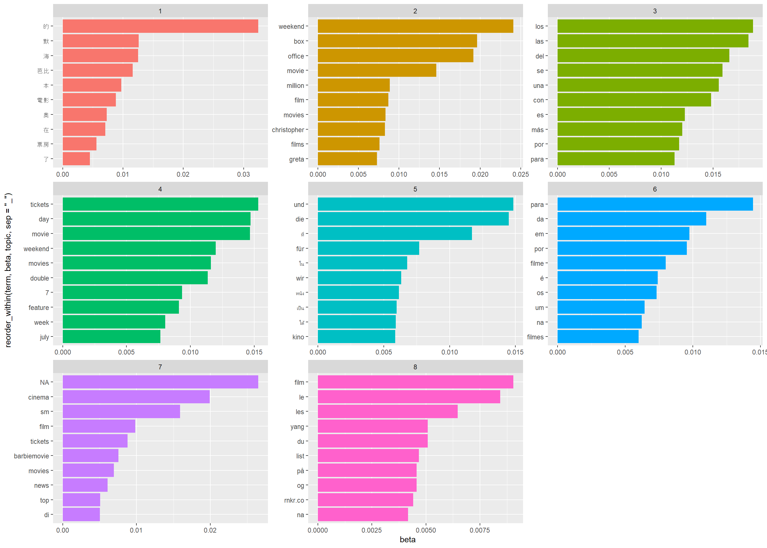
Alright, now that we know how to identify the most meaningful words in a topic, let’s move onto classifying our documents. For this, we’ll want to look at the gamma matrix.
22.2.1.1 gamma
Like beta, we will extract this using the tidy() function.
If you View() this data frame, you’ll notice that each row has the document ID, the gamma number, and the topic. It’s hard using this structure to see how each document is a proportion of each topic, so let’s pivot_wider() this data frame.
topics_wide <- topics_doc %>%
  pivot_wider(names_from = topic,
              values_from = gamma)
#View(topics_wide)
Now, if you view the topics_wide data frame, you can see that each document has a gamma score for each topic. Some gamma scores are larger than others. This suggests that a document’s content is predominantly in one topic as opposed to another.
But sometimes, you want to assign a topic to each document. You can do this by choosing the topic with the highest gamma for each document.
We’ll do this using the slice_max() function in dplyr, which will subset the rows with the largest gamma (per document).
toptopics <- topics_doc %>%
  group_by(document) %>%
  slice_max(gamma)

colnames(toptopics)[1] <- "index"
colnames(toptopics)[2] <- "topics"
toptopics$index <- as.numeric(toptopics$index)
We can then join this data with the full twitter data using full_join(). For this to work, it is essential that your document id is the same id as the status_id in the Twitter data frame. This is why it is essential for you to use the same id’s across all your data analysis. When you use LDA() or when you pivot data, this id wll turn into a character, so make sure to turn it back into a numeric, which is how status_id is normally stored in the data_fb.
We can then plot this information to see which topics have been assigned to the most articles.
table(data_fb2$topics) %>% as.data.frame() %>%
  ggplot(aes(x = Var1, y = Freq)) +
    geom_bar(stat = "identity")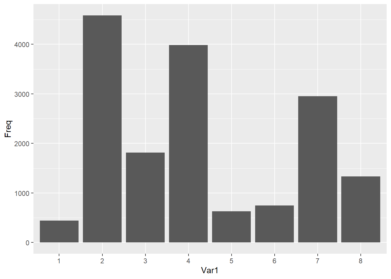
22.3 Bonus: Choosing the K
This analysis should lead you to ask, “okay, but how do we know what is the right number of topics to pick?” For this, the FindTopicsNumber() function in ldatuning can be helpful. FindTopicsNumber() uses a couple of different metrics (four, to be specific). Learn more about each one from their citations:
- Griffiths, T. L., & Steyvers, M. (2004). Finding scientific topics. Proceedings of the National academy of Sciences, 101(suppl 1), 5228-5235.link
- Cao, J., Xia, T., Li, J., Zhang, Y., & Tang, S. (2009). A density-based method for adaptive LDA model selection. Neurocomputing, 72(7-9), 1775-1781.link
- Arun, R., Suresh, V., Madhavan, C. V., & Murthy, M. N. (2010, June). On finding the natural number of topics with latent dirichlet allocation: Some observations. In Pacific-Asia conference on knowledge discovery and data mining (pp. 391-402). Springer, Berlin, Heidelberg.link
- Deveaud, R., SanJuan, E., & Bellot, P. (2014). Accurate and effective latent concept modeling for ad hoc information retrieval. Document numérique, 17(1), 61-84.link
FindTopicsNumber() works by constructing a model for each topic size (in our case, we will use 2 to 20 in iterations of 5). This is sometimes known as the k number of topics. For this reason, this function can take a really long time.
#install.packages("ldatuning")
library(ldatuning)

start_time <- Sys.time() #captures the start of this chunk
result <- FindTopicsNumber(
  data_dtm,
  topics = seq(from = 2, to = 20, by = 5),
  metrics = c("Griffiths2004", "CaoJuan2009", "Arun2010", "Deveaud2014"),
  method = "VEM",
  control = list(seed = 381),
  mc.cores = 2L
)

Sys.time() - start_time #subtracts the current time to the start time to figure out how long this chunk took
## Time difference of 9.796319 minsFinally, we can use the FindTopicsNumber_plot() to plot the results of this analysis. For some of these metrics, the goal is to have a larger measure and for others, the goal is to minimize the measure. FindTopicsNumber_plot() makes it easier to interpret by splitting the maximizing measures and minimizing measures into two charts.
## Warning: The `<scale>` argument of `guides()` cannot be `FALSE`. Use "none" instead as of ggplot2 3.3.4.
## i The deprecated feature was likely used in the ldatuning package.
##   Please report the issue at <]8;;https://github.com/nikita-moor/ldatuning/issueshttps://github.com/nikita-moor/ldatuning/issues]8;;>.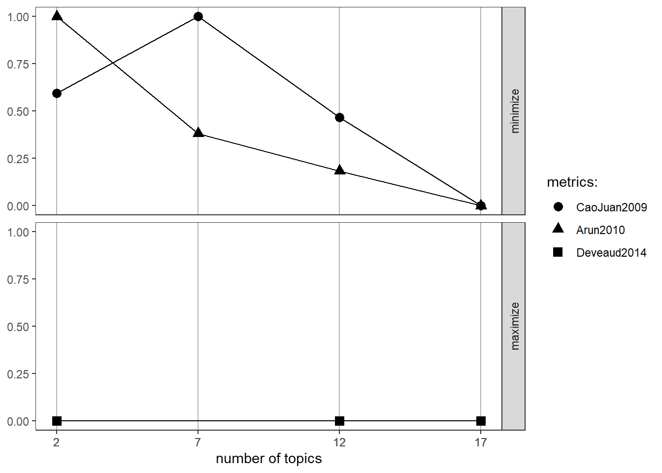
Want more practice with LDA topic modeling? Check out these tutorials:
- Towards Data Science Tutorial, with word clouds link
- Topic Modeling with the textmineR package
- A more in-depth tutorial on the topicmodels package link
- Topic Modeling Video by Julia Silge, tidytext package maintainer video
- Topic Modeling in Quanteda