Chapter 18 Semantic Network Analysis
Hello! In this tutorial, we will be talking about semantic network analyses. These are a special type of analysis that looks at language through the perspective of a network. While there are many ways to construct a semantic network, we will focus on two: a network based on word co-occurances and a network based on bigrams.
To do this, we’ll use a couple of packages. These should mostly be familiar to you from the Week 8 and Week 9 tutorials. The exception to this is widyr, which is used to tidy data into a wide format. widyr has a useful function for analyzing word co-occurrences.
library(tidyverse)
library(tidytext)
library(igraph)
library(ggraph)
library(plyr)
library(widyr) #you may need to install this

set.seed(381)
For this tutorial, we’ll use the rtweet_academictwitter_2021.csv dataset, which we used for our NLP tutorial. Let’s also just focus on the unique tweets.
tw_data_all <- read_csv("data/rtweet_academictwitter_2021.csv")

tw_data <- tw_data_all[!duplicated(tw_data_all$text),]
Let’s start with the bigram network.
18.1 Bigram Network
If you recall from our tidytext tutorial, we can construct bigrams using the tidytext::unnest_tokens() function. Let’s also apply a stop words dictionary to exclude function works and other words with little information. We may want to tailor our stop words list a little more by adding custom words to the pre-existing stop words list. For example, I include the hashtag “academictwitter” because this is the term I searched by in rtweet
final_stop <- data.frame(word = c("academictwitter", "u", "https", "t.co", "n"),
                         lexicon = "custom") %>%
  rbind(stop_words) #adds custom words to stop list
(This is a review.) Bigrams are words that occur in succession (e.g., in “President of the United States,” “President of” is a bigram, “of the” is another bigram, “the United” is a third bigram, and so on). To make sure we remove all the stop words ysed we will construct bi-gram tokens, separate the words, and filter out rows in which the one of the words is in the final stop word list.
tweet_bigram <- tw_data %>%
  unnest_tokens(bigram, text, token = "ngrams", n = 2) %>%
  separate(bigram, c("word1", "word2"), sep = " ") %>%
  filter(!word1 %in% final_stop$word) %>% #uses the combined preset and custom list
  filter(!word2 %in% final_stop$word)

tweet_bigram_ct <- tweet_bigram %>% dplyr::count(word1, word2, sort = TRUE)
head(tweet_bigram_ct, 20)
## # A tibble: 20 x 3
## word1 word2 n
## <chr> <chr> <int>
## 1 phdchat phdlife 130
## 2 academicchatter phdchat 115
## 3 academicchatter openacademics 87
## 4 phdlife phdchat 87
## 5 openacademics academicchatter 64
## 6 academicchatter phdlife 55
## 7 phdchat academicchatter 50
## 8 covid 19 47
## 9 academicchatter academicchatter 45
## 10 0001f4f0 read 42
## 11 malta university 42
## 12 maltauniversity news 42
## 13 student newspoint 42
## 14 um malta 42
## 15 university maltauniversity 42
## 16 phd phdchat 39
## 17 phd students 38
## 18 phdlife academicchatter 37
## 19 phd student 36
## 20 social media 35Nice!
18.1.1 Plotting
How that we have our bigram list, let’s plot this as a network. To do this, we can use the graph_from_data_frame() function we learned in the network analysis tutorial.
tw_bigram_graph <- tweet_bigram_ct %>%
  filter(n > 10) %>% #removes bigrams that appear fewer than 51 times
  graph_from_data_frame()

tw_bigram_graph
## IGRAPH cd02bc3 DN-- 134 133 --
## + attr: name (v/c), n (e/n)
## + edges from cd02bc3 (vertex names):
## [1] phdchat ->phdlife academicchatter->phdchat academicchatter->openacademics phdlife ->phdchat
## [5] openacademics ->academicchatter academicchatter->phdlife phdchat ->academicchatter covid ->19
## [9] academicchatter->academicchatter 0001f4f0 ->read malta ->university maltauniversity->news
## [13] student ->newspoint um ->malta university ->maltauniversity phd ->phdchat
## [17] phd ->students phdlife ->academicchatter phd ->student social ->media
## [21] academicchatter->phdvoice grad ->school commissionsopen->commission university ->science
## [25] mental ->health accept ->rush anthropology ->medtwitter arts ->spiritual
## [29] biology ->neuroscience commisions ->writingcommnunity commission ->commisions grad ->students
## + ... omitted several edgesNow we’re ready to plot this network data!
In addition to using geom_node_point() and geom_edge_link(), we’ll also use the geom_node_text geom to add each word (“name”) as a label for each vertex (“node”),
ggraph(tw_bigram_graph, layout = "fr") + #use the fr layout algorithm
  geom_edge_link() +
  geom_node_point() +
  geom_node_text(aes(label = name),
                 repel = TRUE) + #use repel so the words do not overlap
  theme_void() #void theme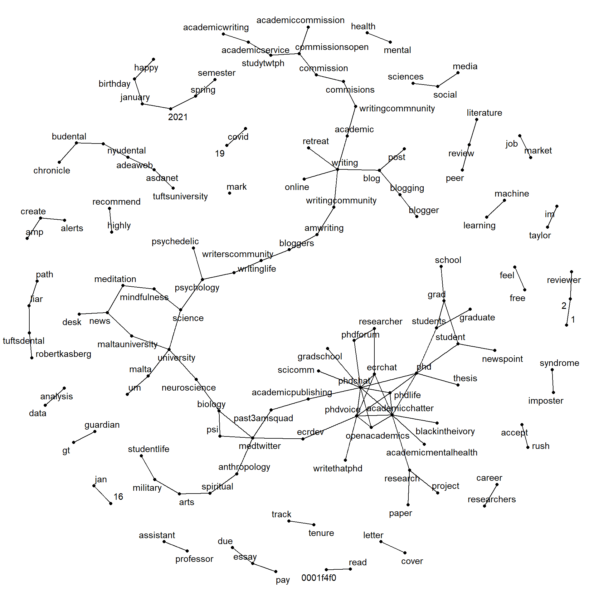
There’s a lot going on here, but we can see that hashtags (academicchatter, mentalhealth, phdchat) and common word-pairs (“reviewer 2” or “writing retreat”) appear in our analysis.
Thus far, we have not used the directional information of the edges. Let’s do that now by adding some grid::arrow() information to geom_edge_link() (the geom that handles edges, or links).
a <- grid::arrow(type = "closed", length = unit(.2, "cm"))
#the above row determines the lay the arrows will look
#check out ?arrow for more information
ggraph(tw_bigram_graph, layout = "fr") + #use the fr layout
geom_edge_link(aes(edge_alpha = n), #vary the edge color by n
#darker lines are bigrams that occur more often
arrow = a, #add the arrow information
) +
geom_node_point(size = 2) + #makes the geom slightly larger
geom_node_text(aes(label = name), #adds text labels for the nodes
repel = TRUE) +
theme_void() #void theme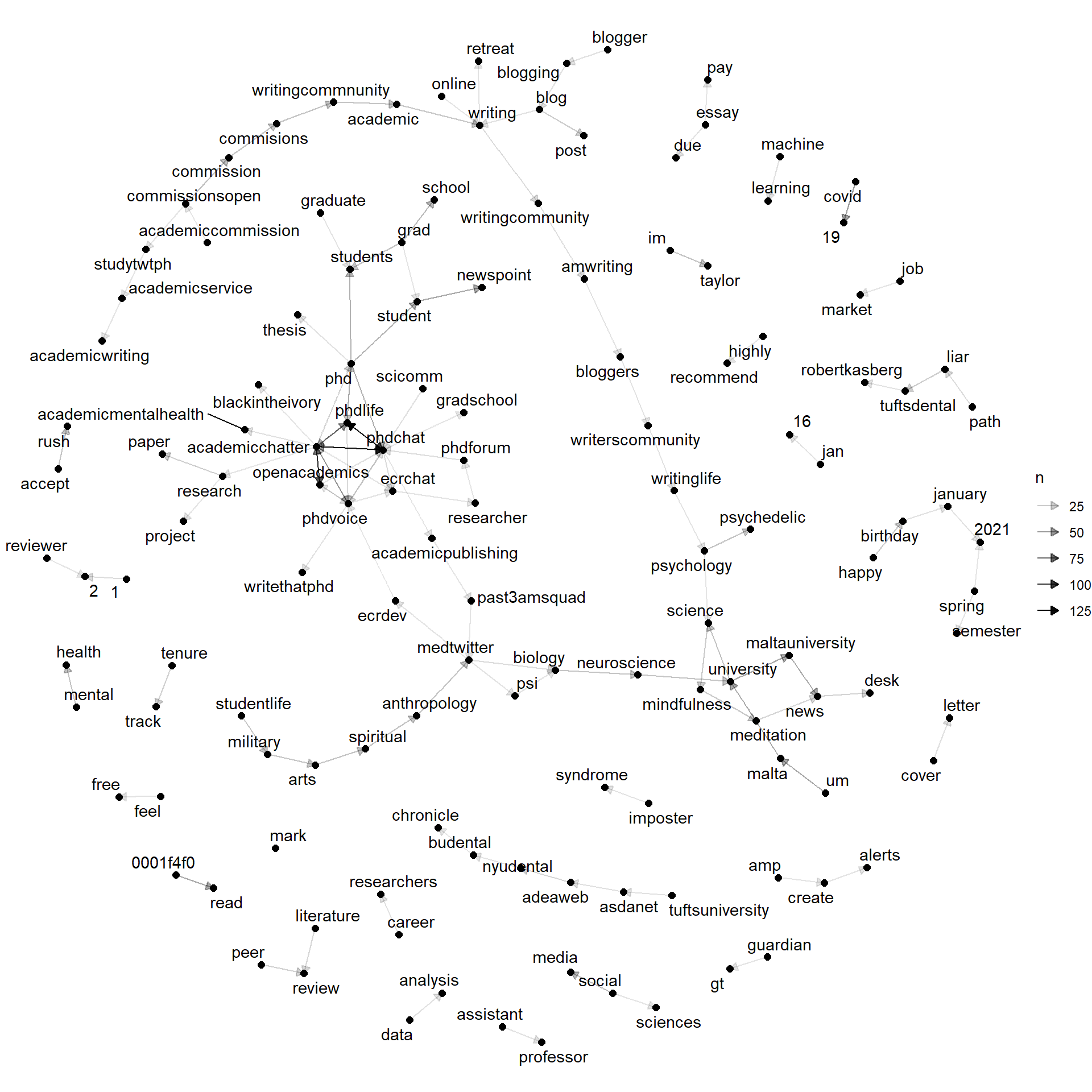 Now, we also know the direction of the bigrams! For example, one of our strongest edges is the one between “phdchat” and “phdlife” (two common hashtags in this community).
Want to learn more about bigram word co-occurrence, check out the fantastic tutorial by Julia Silge.
Let us now turn to the co-occurrence network.
18.2 Co-occurrence Network
In linguistics, two words co-occur if they are likely to appear together in a message (in our case, a tweet). We can plot out a network of word co-occurrences to illustrate which words are used together.
To do this, we’ll tokenize our dataset by word using unnest_tokens(), which we had used previously to make bigram tokens. Now, we’ll use it to make word tokens (recall that “word” is the default token size). Like our other text analysis, we will also remove the stop words using our modified stop words list.
## Joining, by = "word"## # A tibble: 22,822 x 2
## word n
## <chr> <int>
## 1 academicchatter 2180
## 2 phdchat 890
## 3 amp 631
## 4 research 629
## 5 phd 627
## 6 phdlife 504
## 7 students 410
## 8 time 407
## 9 writing 388
## 10 fe0f 375
## # i 22,812 more rowsNow that we have our tokens, let’s calculate their co-occurrence. We can do so using pairwise_count() in the widyr package, which calculates a phi-coefficient. This calculation is similar to the Pearson’s correlation coefficient and, in fact, the phi-coefficient was introduced by Karl Pearson too.
With pairwise_count(), we can calculate if two words co-occur together often using the word itself (word) and an ID for each message (for this, this will be X1).
title_word_pairs <- tw_word_tokens %>%
  widyr::pairwise_count(word, #word data
                        `...1`, #message ID
                        sort = TRUE) #sort the data frame

word_graph <-  graph_from_data_frame(title_word_pairs)

word_graph
## IGRAPH d667576 DN-- 22808 1090120 --
## + attr: name (v/c), n (e/n)
## + edges from d667576 (vertex names):
## [1] phdchat ->academicchatter academicchatter->phdchat phd ->academicchatter academicchatter->phd
## [5] phdlife ->phdchat phdchat ->phdlife phdlife ->academicchatter academicchatter->phdlife
## [9] openacademics ->academicchatter academicchatter->openacademics phd ->phdchat phdchat ->phd
## [13] research ->academicchatter academicchatter->research amp ->academicchatter academicchatter->amp
## [17] phdvoice ->academicchatter academicchatter->phdvoice time ->academicchatter academicchatter->time
## [21] phd ->phdlife phdlife ->phd students ->academicchatter academicchatter->students
## [25] phdchat ->phdvoice phdvoice ->phdchat phdchat ->openacademics openacademics ->phdchat
## [29] academic ->academicchatter academicchatter->academic writing ->academicchatter academicchatter->writing
## + ... omitted several edges18.2.1 Plotting
There are quite a few verticies, so plotting all the verticies would take a long time. Instead, we’ll filter it to the words used more than 50 times.
title_word_pairs %>% #this is our network data
  filter(n >= 40) %>% #which we filter to all co-occurances occurring over 100 times
  graph_from_data_frame() %>% #and then we convert it into a graph
  ggraph(layout = "kk") + #and then we plot a graph with it
    geom_edge_link() + #this graph has an edge geom
    geom_node_point() + #this graph also has a node geom
    geom_node_text(aes(label = name), #we can also add a node text geom to include the word ("name")
                   repel = TRUE) + #use repel to avoid overlapping
  theme_void()
Some things to note from this analysis. First, obviously, hashtags (particularly academicchatter, phdlife, and phdvoice) play a central role in this discourse. We also see some words related to covid, including both covid19 and “covid 19”. However, we do have some noise from this network. For example, there are some encoding issues that ended up in the network (we could add these to the stopwords list so that they are excluded).
Want to play with even more network visuals? Check out this tutorial.