Lesson 2 Data
R is all about data. So let’s look at some! In this lesson, you’ll learn to:
- Import and view a data set.
- Understand the basic vocabulary of data.
- Conduct a short but complete data analysis by compute simple statistics and making a plot.
To start, open RStudio and create a new script for this lesson (calling it, e.g., lesson_data.R, or whatever you want). You’ll use this script to type out some code chunks and see what results they produce.
Then place the following line at the top of your R script, and run it in the console. This will load the tidyverse library, just like we covered in the Libraries lesson:
This will make all the functionality of the tidyverse library available when we need it down below.
2.1 Importing a data set
Let’s see how to import a data set into R. The way I’m going to describe here is very beginner friendly; another (totally optional and more advanced) way is described in “Importing data from the command line.”
Download the data set tvshows.csv, which contains data on 40 shows that aired on major U.S. television networks. A .csv file, like this one, is a common way of encoding tabular data in a way that can be easily shared across platforms.
Important public-service announcement: don’t open that .csv file with Excel first! I see folks do this from time to time in my classes at UT-Austin, and it can produce bizarre errors. Basically, if you open a .csv file with Excel and then hit
Control-Sto save (or let it auto-save), Excel might decide to barf under the rug in your file. This effect will remain insidiously invisible within Excel itself, but can potentially render the file unreadable to RStudio. If you’ve already done this, don’t worry — just delete the file and download a fresh copy.7
This video shows how import a data set into RStudio. But we’ll cover the steps here, too:
- Go to the
Environmenttab in RStudio’s top-right panel.
- Click the
Import Datasetbutton. You’ll see a pop-up menu. Choose the first option:From Text (base)....
- A standard file-browser window should pop up. Use it to navigate to wherever you saved the
tvshows.csvfile. When you find it, clickOpen.
At this point, a new window should pop up that looks something like this. I’ve labeled several parts of this screen shot in red, so that I can refer to them below.
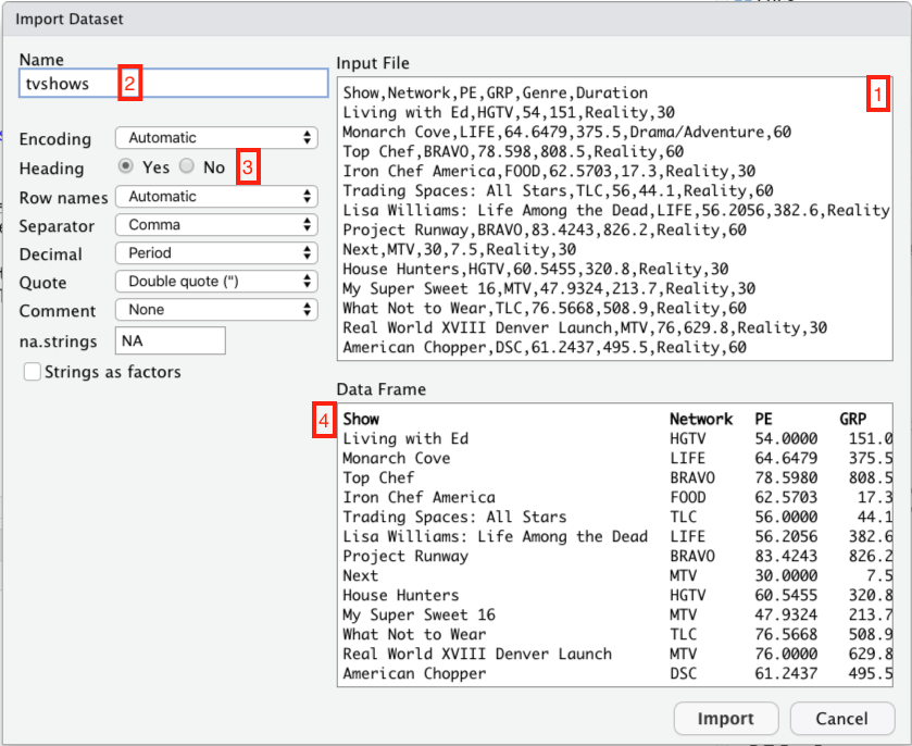
Let’s take those four red boxes in turn:
- This is what the raw .csv looks like. It’s just what you’d see if you opened the file in a plain text editor.
- This is the name of the object in R that will be created in order to hold the data set. It’s how you’ll refer to the data set when you want to do something with it later. R infers a default name from the file itself; you can change it if you want, but there’s usually no good reason to do so.
- This tells R whether the data set has a header row—that is, whether the first row contains the names of the columns. Usually R is pretty good at inferring whether your data has a header row or not. But it’s always a good idea to double-check: click
Yesif there’s a header row (like there is here), andNoif there isn’t.
- This little window shows how the imported data set will appear to R. It’s a useful sanity check. If you’ve told R (or R has inferred) that your data set has a header row, the first row will appear in bold here.
Now click Import. The imported data set should pop up in a Viewer window, like this:
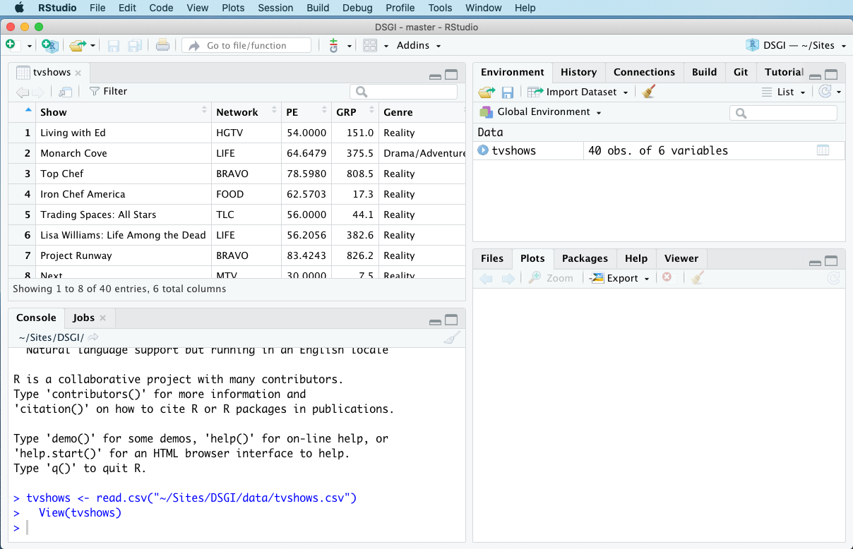
Note that you can’t actually edit the data set in this window—only view it. You may also notice that tvshows is now listed under the Environment tab in the top-right panel. This tab keeps track of all the objects you’ve created.
The Viewer window is a perfectly fine way to look at your data. I find it especially nice for giving me a “birds-eye” view of an unfamiliar data set. If you’ve closed the Viewer window, you can always conjure it back into existence using the view function, like this:
view(tvshows)Another handy “data viewing” command in R is called head. This command will print out the first six of a data set in the console, like this:
##                                 Show Network      PE   GRP           Genre Duration
## 1                     Living with Ed    HGTV 54.0000 151.0         Reality       30
## 2                       Monarch Cove    LIFE 64.6479 375.5 Drama/Adventure       60
## 3                           Top Chef   BRAVO 78.5980 808.5         Reality       60
## 4                  Iron Chef America    FOOD 62.5703  17.3         Reality       30
## 5          Trading Spaces: All Stars     TLC 56.0000  44.1         Reality       60
## 6 Lisa Williams: Life Among the Dead    LIFE 56.2056 382.6         Reality       60
I use this one all the time to get a quick peek at the data, but don’t want the pop-up viewer window to take me away from my script—like, for example, when I need to remind myself what the columns are called.
2.2 The vocabulary of data
Let’s talk about the structure of this tvshows data set, as a way of introducing some important vocabulary terms.
- The typical way R stores data is in a tabular format called a data frame.
- Each row of the data frame is called an example, a case, or an observation. These three words can be used interchangeably. Here, each example is a TV show.
- A collection of examples is called a sample, and the number of examples is called the sample size, usually denoted by the letter \(n\). Here our sample size is \(n=40\).
- Each column of the data frame is called a feature (or sometimes a variable). Each feature conveys a specific piece of information about the examples.
- The first feature,
Show, tells us which TV show we’re talking about. This type of feature is called a unique identifier, or just an ID.
- Some features in the data set are actual numbers; appropriately enough, these are called numerical features. The numerical features in this data set are
Duration,GRP(“gross rating points”, a measure of audience size), andPE(which stands for “predicted engagement” and measures whether the audience is actually paying attention to the show).
- Other features in the data set can only take on a limited number of possible values, just like the answer to a multiple-choice question. The categorical features in this data set are categorical features. The categorical features in this data set are
NetworkandGenre.8
So, for example, a data set with 500 examples and 10 features would be stored in a data frame with 500 rows and 10 columns.
2.3 A short, simple data analysis
Once you’ve imported a data set and comprehended its basic structure (using, e.g., view or head), the next step is to try to learn something from the data by actually analyzing it. We’ll see many ways to do this in the lessons to come! But for now, here’s a quick preview of the two simplest ways: calculating summary statistics and making plots.
A statistic is any numerical summary of a data set. Statistics are answers to questions like: How many reality shows in the sample are 60 minutes long? Or: What is the average audience size, as measured by GRP, for comedies?
A plot, meanwhile, is exactly what it sounds like: per Wikipedia, a “graphical technique for representing a data set, usually as a graph showing the relationship between two or more variables.” Plots can help us answer questions like: What is the nature of the the relationship between audience size (GRP) and audience engagement (PE)?
Let’s see some examples, on a “mimic first, understand later” basis. Just type out the code chunks into your lesson_data.R script and run them in the console, making sure that you can reproduce the results you see below.
Our first question is: how many reality shows in the sample are 60 minutes long, versus 30? As we’ll learn in the upcoming lesson on Counting, the xtabs function gets R to count for us:
##                   Duration
## Genre              30 60
##   Drama/Adventure   0 19
##   Reality           9  8
##   Situation Comedy  4  0
It looks like 8 reality shows are 60 minutes long (versus 9 that are 30 minutes long).
Let’s answer a second question: what is the average audience size for comedies, as measured by GRP? Calculating this summary actually requires multiple lines of R code chained together, and it relies upon functions defined in tidyverse, so it won’t work if you haven’t already loaded that library. You might be able to guess what this code chunk is doing, but we’ll understand it in detail in the upcoming lesson on Summaries.
## # A tibble: 3 x 2
##   Genre            mean_GRP
##   <chr>               <dbl>
## 1 Drama/Adventure     1243.
## 2 Reality              401.
## 3 Situation Comedy     631.
The result is a summary table with one column, called mean_GRP. It looks like comedies tend to have middle-sized audiences: an average GRP of about 630, versus 401 for reality shows and 1243 for drama/adventure shows.
Finally, let’s make a plot to understand the relationship between audience size (GRP) and audience engagement (PE). We’ll make this plot using a function called ggplot, which is made available by loading the tidyverse. Again, don’t sweat the details; we’ll cover ggplot in detail in the upcoming Plots lesson. Just copy/paste the statements into your script, run them, and observe the result:
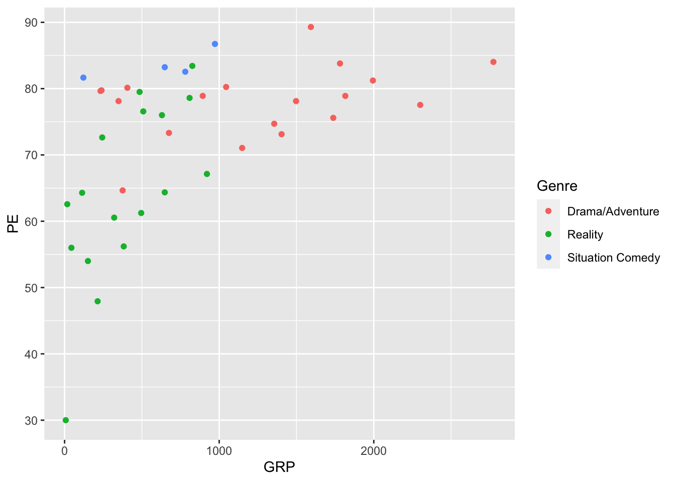
We’ve learned from this plot that shows with bigger audiences (high GRP) also tend to have more engaged audiences (higher PE), a fact that isn’t necessarily obvious (at least to me) until you actually look at the data. If you wanted to save this plot (say, for including in a report or a homework submission), you could click the Export button right above the plot itself and save it in a format of your choosing. You can also click the Zoom button to make the plot pop out in a resizeable window.
Note: this plot above actually isn’t great, because the red and green can look nearly identical to color-blind viewers. I’m especially sensitive to that issue, since I’m red-green colorblind myself.

We’ll clean up that problem in a later lesson, when we learn more about plots. But for now, focus on your victory! You’ve now conducted your first data analysis—a small one, to be sure, but a “complete” one, in the sense that it has all the major elements involved in any data analysis using R:
- import a data set from an external file.
- decide what questions you want to ask about the data.
- write a script that answers those questions by running an analysis (calculating statistics and making plots).
- run the script to see the results.
In the lessons to come, we’re going to focus heavily on the “analysis” part of this pipeline, addressing questions like: what analyses might I consider running for a given data set? How do I write statements in R to run those analyses? And how do I interpret the results?
2.4 Importing data from the command line
This section is totally optional. If you’re an R beginner, or you’re happy with the Import Dataset button for reading in data sets, you can safely skip this section and move on to the next lesson.
If, on the other hand, you have a bit more advanced knowledge of computers and are familiar with the concepts of pathnames and absolute vs. relative paths, you might prefer to read in data from the command line, rather than the point-and-click interface of the Import Dataset button. I personally prefer the command-line way of doing things, because it makes every aspect of a script (including the data-import step) fully reproducible. The downside is that it’s less beginner-friendly.
Let’s see an example. To read in the tvshows.csv file from the command line in R, I put the following statement at the top of my script:
This statement reads the “tvshows.csv” file off my hard drive and stores it in on object called tvshows. Let’s break it down:
read.csvis the command that reads .csv files. It expects the path to a file as its first input.
'data/tvshows.csv'is the path to the “tvshows.csv” file on my computer. In this case it’s a relative path (i.e. relative to the directory on my computer containing the R file from where the command was executed). But you could provide an absolute path or a url instead.
header=TRUEtells R that the first row of the input file is a header, i.e. a list of column names.
tvshowsis the name of the object we’re creating with the call toread.csv. It’s how we’ll refer to the data set in subsequent statements.
R has a whole family of read functions for various data types, and they all follow more or less this structure. I won’t list them all here; this overview is terse but authoritative, while this one is a bit friendlier-looking.
In my experience this behavior seems to depend on your platform and version of Excel. It is possible to safely open and edit .csv files within Excel, but then you have to re-export them as .csv files again if you want to use them in RStudio.↩︎
You could also argue that
Duration, despite being a number, should really be considered a categorical feature, since it only takes on a set of specific values like 30 and 60.↩︎