12 Specification curve analysis
12.1 Introduction: The garden of forking paths
When you analyse a dataset, you have many choices in how to specify your statistical model. Let’s think back to the “tomboys” data set from the last session (Atkinson, Smulders, and Wallenberg 2017). The authors were interested in whether someone was a tomboy or not, so the outcome variable (called yesOrNo in the data set, 1 for was called a tomboy, 0 for not) is pretty clear. But there are actually several ways they could have tested the hypothesis that they stated.
First, there is the 2D:4D ratio. They measured both hands. So, they could use the ratio for the right hand; or the ratio for the left hand; or, the average of the ratios of the right and left hands (these variables are all in the data set, variables rightHand, LeftHand and Averagehand respectively). So the first forking path in the garden is which hand to use.
Then, there is the decision of whether to log transform whichever 2D:4D we settle on. The authors looked at the distribution and decided they should, but they might not have log transformed, and that would have seemed a reasonable decision too.
Also in the paper, the authors consider whether the covariates Age and Ethnicity might need to be included. In fact there are four possibilities as far as covariates are concerned: include neither Age nor Ethnicity; Age but not Ethnicity; Ethnicity but not Age; or include both Age and Ethnicity .
So, when we think about it, there are actually 24 ways the data could have been analysed to test the prediction (at least, there are probably other variants too that we have not discussed). The 24 number comes from: 3 different 2D:4d measures, times 2 for either log transforming or not, times 4 for the combinations of covariates included or not included.
Now, this is a problem, because every one of those 24 ways represents another ‘go’ at getting a significant p-value. Obviously, if you run enough tests, some of them will come up significant, even if the hypothesis is false (by definition, one in 20 will if the threshold is p = 0.05). The researchers are presenting us with only some of the 24 possible model specifications, finding a ‘significant’ result (p just a bit less 0.05). We really want to know which of the following situations we are in. Is it (a) any of the 24 possible specifications would lead to conclusion of a significant association between tomboy status and 2D:4D; (b) only a very few of the 24 possible specifications would lead to the conclusion of a significant association; or (c) somewhere in between, a good number but not all of the specifications would lead to the conclusion of a significant association.
If we are in world (a), then we really believe that the result is probably not a fluke. We would have come to the same conclusion however we had specified our model. If we are in world (b), only a few specifications produce the conclusion, we should be more alert to the possiblility that the association is a kind of fluke: you only infer the effect under very specific modelling assumptions, and it disappears when those assumptions are permuted in any way. And if we are in world (c), then it is interesting to know what proportion of possible specifications lead to the same conclusion, and which modelling choices make the difference. This information is really going to help us evaluate the strength of the evidence presented. For this reason, one of the principles of sound data analysis that I mentioned in section 8.5 is that sensitivity to analytical decisions has been explored.
12.1.1 The traditional way of dealing with flexibility in specification
Researchers have known for ever that some conclusions are changed by altering the specification of the model, and that it is important to communicate the extent to which this is the case. For this reason, papers will often play about with different specifications to convince you that specification choices don’t matter for the conclusions. In the paper on the tomboy study, for example, they start by presenting a simple model just using the logged right hand variable, then they experiment with adding age and show that makes no difference, and then they experiment with adding ethnicity (without age) and show this makes no difference either. Finally, they mention that you don’t get the same conclusion by using the left hand. What they don’t do, however, is systematically try out all the logically possible combinations.
You will often read papers that present a model 1, with no covariates, and then a model 2 that adds some more, a model 3 that adds still more, and so on. But this is still a rather improvised way of exploring sensitivity of conclusions to analytical decisions. A more modern way is called specification curve analysis (also known as multiverse analysis), and it is what we are going to do today.
12.1.2 Principles of specification curve analysis
The principle of specification curve analysis is actually very simple. You work out the total set of model specifications that you might have presented and it felt reasonable. For example, here, we have the 24 possibilities made up by the combinations of which hand to use, whether or not to log transform, and which set of covariates to include. Then, you run all 24 of these models, and you visualize what the parameter estimates and their confidence intervals are for each one. In particular, this allows you to identify which features of the specification matter for the parameter estimate. For example, log transforming the outcome variable might be critical to your conclusion, but including age as a covariate might make no difference at all. In the next section, we will run a simple specification curve analysis for the tomboy data.
12.2 Running a specification curve analysis
12.2.1 Load in the tomboy data, again, and get the “specr” package
Let us start by reading in the tomboy dataset that we used last time.
library(tidyverse)
t <- read_csv("https://raw.githubusercontent.com/joelcw/gendocrine/refs/heads/master/datasets/tomboys.csv")
## Rows: 46 Columns: 20
## ── Column specification ──────────────────────────────────
## Delimiter: ","
## chr (3): Participant, id, Ethnicity
## dbl (17): Masculine, Feminine, SRIRatio, Androgynous, ...
##
## ℹ Use `spec()` to retrieve the full column specification for this data.
## ℹ Specify the column types or set `show_col_types = FALSE` to quiet this message.For specification curve analysis, we are going to use a contributed package called specr, so let’s install it and activate it in this session.
12.2.2 How specr works: Specifying you specifications
To make the specr package do its thing, you need to be able to define some features of the set of possible specifications:
What were all the possible outcome variables (
specrcalls these y variables; here, only one,yesOrNo);What were all the possible predictor variables (
specrcalls these x variables;here, remembering I always like to scale predictors, we havescale(rightHand),scale(log(rightHand)),scale(LeftHand),scale(log(LeftHand)),scale(AverageHand)andscale(log(AverageHand));What were all the possible covariates (
specrcalls these controls; here,AgeandEthnicity);Were there any subsets of the data we might have used (I don’t think so in this case);
What are all the kinds of models we might want to fit (here, only really the Generalized Linear Model of the binomial family, I don’t think there is any other reasonable choice).
You feed all this information to a function called setup(), which then work out all the possible specifications.
There is one slightly tricky aspect to using specr in this particular case, which is that our Generalized Linear Model of the binomial family is not something it recognises automatically. We have therefore to write a user-defined function for fitting this class of model. Don’t worry too much about this bit, it is just to make setup() work with our model, but you do need to run it before you can get any further, trust me. If our model was a simple lm() we would not need to be doing this step.
Ok, so now we call the setup function:
specs <- setup(data=t,
               y = "yesOrNo",
               x = c("scale(lnRight)",
                     "scale(rightHand)",
                     "scale(lnLeft)",
                     "scale(LeftHand)",
                     "scale(log(Averagehand))",
                     "scale(Averagehand)"),
               controls=c("Age", "Ethnicity"),
               model = "glm_binomial")
As you can see, what we are doing here is listing all the possibilities for the y variable, the x variable, the controls and the kind of model (glm_binomial calls back to the user-defined function I made in the previous chunk of code).
Now we can ask for a summary of our specs object:
## Setup for the Specification Curve Analysis
## -------------------------------------------
## Class:                      specr.setup -- version: 1.0.0
## Number of specifications:   24
##
## Specifications:
##
##   Independent variable:     scale(lnRight), scale(rightHand), scale(lnLeft), scale(LeftHand), scale(log(Averagehand)), scale(Averagehand)
##   Dependent variable:       yesOrNo
##   Models:                   glm_binomial
##   Covariates:               no covariates, Age, Ethnicity, Age + Ethnicity
##   Subsets analyses:         all
##
## Function used to extract parameters:
##
##   function (x)
## broom::tidy(x, conf.int = TRUE)
## <environment: 0x000001c80da5b218>
##
##
## Head of specifications table (first 6 rows):
## # A tibble: 6 × 6
## x y model controls subsets formula
## <chr> <chr> <chr> <chr> <chr> <glue>
## 1 scale(lnRight) yesOrNo glm_b… no cova… all yesOrN…
## 2 scale(lnRight) yesOrNo glm_b… Age all yesOrN…
## 3 scale(lnRight) yesOrNo glm_b… Ethnici… all yesOrN…
## 4 scale(lnRight) yesOrNo glm_b… Age + E… all yesOrN…
## 5 scale(rightHand) yesOrNo glm_b… no cova… all yesOrN…
## 6 scale(rightHand) yesOrNo glm_b… Age all yesOrN…So, we can see that there are 24 specifications, and the first 6 are listed for us.
12.2.3 Running the analysis
Now that we have set up our set of specifications, it is time to run the specification curve analysis, using the function specr(). We do this as follows:
Now, you will probably get some scary warning messages here. These are however just courtesy warnings, and they have not stopped the models being fitted. Much the best way to examine the output of specr() is to plot results.
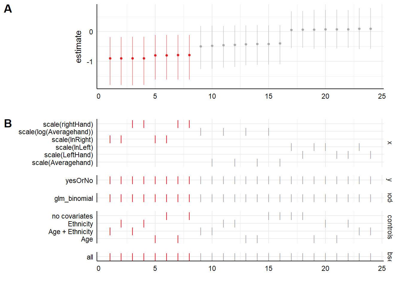
Plot A shows us the parameter estimates for the effect of the x variable on the y variable, for each of the 24 specifications. The ones in red show an association that is significantly different from zero, whilst the ones in grey show those whose confidence intervals overlap zero. As we see, the first eight specifications show our significant negative association, and the next sixteen do not, they show associations around zero.
Plot B shows you what is in each of the specifications in the plot above, showing a tick where a variable is present. So as you can see, the first eight are the specifications that use the right hand 2D:4D. All of these find the significant associations. In fact, within these eight, it makes remarkably little difference whether we log transform or not, and which covariates we include.
The next sixteen either use average hand, or left hand. As you can see, those using left hand produce no hint of a negative association. As you might expect, the parameter estimates for average hand are intermediate between those for left hand and those for right hand (but, not significantly different from zero). Within the sets using left hand or right hand, again, the decision to log transform or not, or to include covariates or not, makes no perceptible difference.
12.2.4 So what do we conclude in this case?
The conclusion from this specification curve analysis is very clear. The claims made in the paper are totally robust to assumptions about log transforming the predictor variable and the inclusion of covariates. Researchers could make any decision in these dimensions and would still come the same conclusion. This is reassuring.
On the other hand, the claims are totally dependent on using the right hand for the 2D:4D measurement, not the left hand or the average of the two hands. If the researchers made a different decision here, the conclusion would be no association.
Now, the researchers do acknowledge in the paper that they only find the association using the right hand. Indeed, they cite previous studies also suggesting that it is the right hand that best reflects in utero testosterone, so this makes sense. How you evaluate this is up to you. They did not pre-register that it would be the right hand, not the left, that would predict being a tomboy. And they measured the left hand. And they calculated the average of the two hands as well. So, did they genuinely have an a priori expectation that the right hand 2D:4D but not the left would predict being a tomboy? Or did they try everything and hypothesize after the result was known? We can’t tell. This is one of the reasons why preregistration is so good. It allows us to be clear about which are genuinely prior expectations, and which are just things that make sense after the fact.
In any event, the specification curve analysis neatly shows under what set of specifications you get to the published conclusion, and under what set you do not. This helps us refine our expectations (and plan our analysis strategies) for future confirmatory studies based on these findings.
12.3 How to use and report specification curve analysis
Specification curve analysis often involves many more specifications than the 24 used in the example above, sometimes even thousands. It is a very handy way of showing the robustness of conclusions and being transparent about their limits. I would recommend using it as a supplement to your preregistered analysis in all preregistered studies; and in all cases for exploratory studies.
The key step in doing a specification curve analysis is working out what your possible universe of specifications is. It can only include specifications that are still tests of the same research question. Sometimes in a study when we report an additional specification, it is not as additional test of the same question, but as an approach to a novel follow up question. For example, we might be wanting to know about a mediator or moderator variable. These kinds of question-changing analysis are not in the same set for specification curve analysis, because they are not tests of exactly the same question.
Also, your set of specifications for a specification curve analysis should only include specifications that actually seem reasonable. There is no interest in showing that hundreds of bad specifications that no reasonable person would ever propose lead to null conclusions. Rather, you are trying to identify the set of specifications that you (or another researcher) might reasonably have thought to try in pursuit of the same question.
You might use the information from the specification curve analysis in a number of different ways. These vary a bit depended on whether your analysis plan is preregistered or not, and at what stage you bring the specification curve analysis in.
If you are preregistering an analysis plan, you might realise that there are several ways of doing the analysis that are equally reasonable a priori. In this case, you could preregister that you will do all of them and plot a specification curve analysis. In the interests of comprehensibility as much as anything else, I would recommend choosing one specification as primary, but preregistering that you will run all the others to investigate the robustness of the conclusion. Of course this slightly raises the issue of what to conclude if the one you preregistered as primary produces one conclusion whereas other specifications produce different ones. This means that the results of your study are not very robust to choice of specification; but at least with the specification curve analysis, this will be clear and transparent.
If you have already preregistered an analysis plan, in the course of the analysis you might realise that there were other specifications that you could have chosen to use (or that other researchers or reviewers might have preferred), but you did not preregister them. Here, I would put a specification curve analysis in an appendix to show to what extent specification choices might make a difference. I would still report my preregistered analysis as primary in the main text, unless there was some strong justification for departing from it, which you would have to explain.
If your study is not preregistered at all, then it is particularly important to do a specification curve analysis. To help the reader, again, I would probably start by presenting a main specification, but then, either in the main text or an appendix, show how robust this is to reasonable departures from the specification.