11 Generalized Linear Models
11.1 Introduction To Generalized Linear Models
When we have modeled data so far, we have had a continuous outcome variable. This has allowed us to set up a General Linear Model where the outcome variable is expressed as the sum of the predictor variables, each weighted by the relevant parameter estimate, plus a Normally distributed error term. Where we have just one predictor variable, this looks as follows:
\[ y_i = \beta_0 + \beta_1*x_i + \epsilon_i \\ \epsilon \sim N(0, \sigma^2) \]
What though if our outcome variable is not continuous? Consider for example the case where our outcome variable is something that either happens or does not (i.e. is binary, with 0 representing the outcome not happening and 1 representing the outcome happening).
Here, the General Linear Model above does not seem to fit the situation too well. If you look at the structure of the linear predictor part in the equation, \(\beta_0 + \beta_1 * x_i\), this implies that as the \(x\) gets bigger, then the predicted value of \(y\) will get bigger too, in a straight-line fashion (assuming \(\beta_1\) is positive). There is no upper limit to this assumed linear relationship; for any value of \(x\), adding a further 1 to it will cause \(y\) to get bigger, by an amount \(\beta_1\). But our outcome variable in the current case can’t go on getting bigger as the predictor variable gets bigger: \(y\) can only happen rather than not happening. The probability of \(y\) happening is bounded at 1, and at 0, so a linear relationship between the value of \(x\) and the value of \(y\) extending indefinitely in both directions is not the right assumption. The errors are also unlikely to be Normal in this case, again because they are bounded. The prediction cannot be more wrong than predicting the event will definitely happen when in fact it does not (error value -1), or predicting that it definitely won’t happen when in fact it does (error +1).
We solve this problem by selecting a model from a broader class of models than the General Linear Model with Normal errors that we have encountered so far. The broader class is called the Generalized Linear Models. (In fact, the General Linear Model we have used so far belongs to the broader Generalized class; the point is that it is only one member of that class, and there are others available.)
In Generalized Linear Models, we have an outcome variable \(Y\) and some set of predictors \(X_1, X_2,...\), as before. Rather than predicting the value \(y\) from the weighted sum of the predictors, we are going to predict some function of \(y\) from the predictors. The function chosen is called the link function and I will say more about it below. The other innovation in Generalized Linear Models is that the distribution of errors need not be assumed to be the Normal distribution. There are other options such as the Poisson or binomial distributions. The combination of which link function and which assumed error distribution we choose defines the family that our Generalized Linear Model belongs to.
Today we will work with a Generalized Linear Model suitable for the case where the response variable is binary. This means we want a model of the binomial family of Generalized Linear Models. Models of this family assume a logit function as the link function, and a binomial distribution for the error term.
The logit link function means that we are assuming that what changes as the values of the predictors change is the log odds of the outcome happening. To understand what this means, we need to first explain odds. The odds of an outcome happening are defined as: \[ \frac{p}{1-p} \]
Here, \(p\) is the probability of the outcome happening. So, if the outcome has a 50% chance of happening, its odds are 1; if it has a 90% chance of happening, they are 9; and if it has a 10% chance of happening, they are \(\frac{1}{9}\). Odds are bounded at zero, if the outcome will never happen, and approach infinity as the outcome approaches certainty. The log odds is just the logarithm of the odds. The log odds is bounded at minus infinity and infinity, with zero reflecting even odds (because if the probability of the event is 50%, the odds are 1, and the log odds is thus 0). If the log odds gets bigger, the odds of the outcome get bigger, and so the probability of the outcome gets bigger. If the log odds gets smaller, the odds of the outcome get smaller, and so the probability of the outcome gets smaller.
Let’s denote the log odds of the outcome as \(\lambda(y)\). Our Generalized Linear Model assumes a relationship between the predictors and the outcome as follows: \[ \lambda(y) = \beta_0 + \beta_1 * x + \epsilon \]
In other words, the log odds of the outcome \(Y\) happening have some baseline level \(\beta_0\), and increase by a factor of \(\beta_1\) for every unit change in the predictor variable \(X\). Of course, \(\beta_1\) could be zero, meaning that \(X\) has no predictive power for the odds of \(Y\) occurring; or positive (meaning a higher value of \(X\) increases the odds of \(Y\) occurring); or negative (meaning a higher value of \(X\) decreases the odds of \(Y\) occurring). Remember that \(\beta_1\) (along with its standard error) will be estimated from the data.
This will become clearer when we do it, so let’s turn to an empirical example.
11.2 Introducing a new dataset: Atkinson, Smulders and Wallenberg (2017)
11.2.1 The “tomboy”study
We are going to work with the data from a paper on pre-natal exposure to testosterone and “tomboy” identity in girls (Atkinson, Smulders, and Wallenberg 2017). The paper is published in a paywall journal (boo!) but there is a free PDF version available at: https://eprints.ncl.ac.uk/231669.
“Tomboys” are girls who get identified, usually by their parents, as having boy-like or male-typical interests or behaviours. The hypothesis of the study was that exposure to higher levels of testosterone in utero will make a girl more likely to develop male-typical interests and behaviours, and hence more likely to end up being recognised as a “tomboy”. Fortunately, there is a proxy which is supposed to capture what level of testosterone you were exposed to in utero. This variable is the ratio of the lengths of the second to fourth finger of the right hand (the 2D:4D ratio). A lower 2D:4D ratio is supposed to indicate exposure to higher levels of testosterone in utero (how credible you find the whole study will depend on how credible you find the 2D:4D ratio as a proxy for in utero testosterone). Thus, the hypothesis of the study is that a continuous variable, right hand 2D:4D ratio, will predict a binary outcome, namely answering “Yes, I was called a tomboy when I was a girl”, or “No, I was not called a tomboy”. The participants are all adult women by the time of the study. Because we have a continuous predictor and a binary outcome, this dataset is perfect to try out a Generalized Linear Model of the binomial family.
11.2.2 Getting the data
The data for the study are published online on a repository called Github, and there is a link in the paper. If you click on the link you will see the data. To take the data off and into R, the URL you need is for the “raw” version, and hence not the exact URL given in the paper. I have given you the link in the code below. We are going to call our data frame t for a change.
library(tidyverse)
t <- read_csv("https://raw.githubusercontent.com/joelcw/gendocrine/refs/heads/master/datasets/tomboys.csv")
## Rows: 46 Columns: 20
## ── Column specification ──────────────────────────────────
## Delimiter: ","
## chr (3): Participant, id, Ethnicity
## dbl (17): Masculine, Feminine, SRIRatio, Androgynous, ...
##
## ℹ Use `spec()` to retrieve the full column specification for this data.
## ℹ Specify the column types or set `show_col_types = FALSE` to quiet this message.Now let’s have a look at what our data frame contains:
##  [1] "Participant" "Masculine"   "Feminine"
##  [4] "SRIRatio"    "Androgynous" "RIGHT"
##  [7] "LeftHand"    "Averagehand" "Identity"
## [10] "Kinsey"      "Age"         "Tomboy"
## [13] "yesOrNo"     "zAge"        "rightHand"
## [16] "lnRight"     "lnLeft"      "test"
## [19] "id"          "Ethnicity"
This dataset is a bit of a mess, by the way. The variables are not consistently labelled: LeftHand, which is the left hand 2D:4D ratio starts with a capital letter, rightHand does not start with a capital, and the rightHand variable is repeated with a different name RIGHT. There are three different variables that represent the outcome: Tomboy codes 1 for tomboys and 2 for not tomboys; yesOrNo codes tomboys as 1 and not tomboys as 0; and id codes the same information in words. Please don’t do this kind of stuff. Have comprehensible labels, the minimum number of columns, and use capitalization consistently. Try to be clear and consistent for your readers.
We want the outcome variable coded as 1, was identified as a tomboy, or 0, was not, so we will use the variable yesOrNo. As for the predictor, the authors suggest in the paper that the right hand 2D:4D should be logged as it shows a skewed distribution.
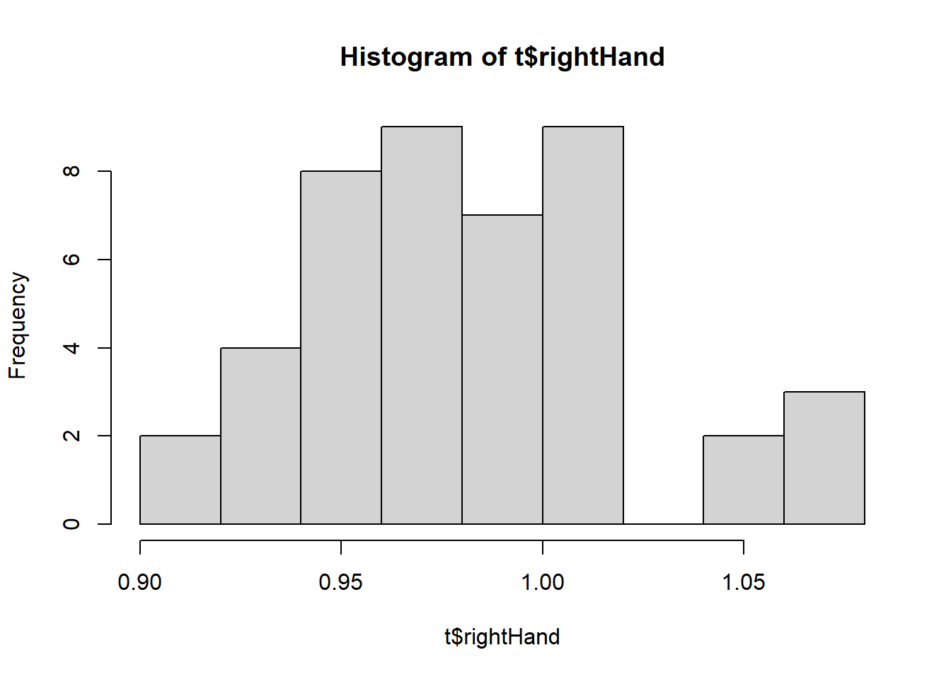
I don’t actually think it’s too bad, but we will follow what they did in the paper (it makes no difference, actually). The authors have provided a logged version already in the data frame (variable lnRight). You could also calculate your own if you wanted to:
The log() function in R makes natural logs (base e) by default.
11.2.3 Checking and a quick plot
Let’s have a quick look at what is in the data.
##
##  0  1
## 26 20
It looks like we have 20 women who were identified as tomboys, and 26 who were not. If the hypothesis of the study is supported, the tomboys will have lower lnRight than the non-tomboys. Let’s have a quick look:
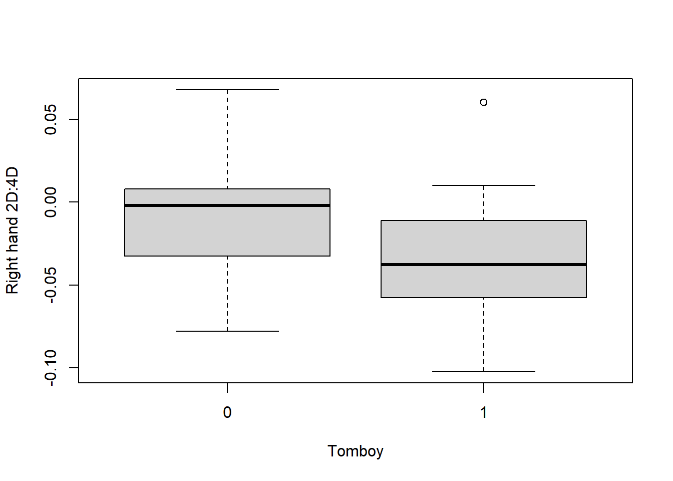
It looks like the hypothesis might be supported. So, it’s time to test this properly with our Generalized Linear Model.
11.3 Fitting the Generalized Linear Model
The function we need for our Generalized Linear Model is glm(). The syntax is much the same as the lm() function we have already used, with the additional step that you need to specify the family of your model (here, binomial). So, let’s fit the model. We will just use the most simple possible version at first (i.e. not controlling for any covariates). As before, I am going to scale my continuous predictor variable. They did not do this in the original paper, which is why the magnitude of the reported parameter estimate in their paper is not going to be the same as the one you get here (though the direction of the relationship and its statistical significance are the same).
##
## Call:
## glm(formula = yesOrNo ~ scale(lnRight), family = "binomial",
##     data = t)
##
## Coefficients:
##                Estimate Std. Error z value Pr(>|z|)
## (Intercept)     -0.3198     0.3266  -0.979   0.3274
## scale(lnRight)  -0.7950     0.3730  -2.131   0.0331 *
## ---
## Signif. codes:
## 0 '***' 0.001 '**' 0.01 '*' 0.05 '.' 0.1 ' ' 1
##
## (Dispersion parameter for binomial family taken to be 1)
##
##     Null deviance: 60.176  on 43  degrees of freedom
## Residual deviance: 54.715  on 42  degrees of freedom
##   (2 observations deleted due to missingness)
## AIC: 58.715
##
## Number of Fisher Scoring iterations: 4
Right, we seem to have a significant (p < 0.05) association between the right hand 2D:4D and being a tomboy, with a negative coefficient (-0.795). We can also get the confidence intervals on this parameter estimate:
## Waiting for profiling to be done...## 2.5 % 97.5 %
## (Intercept) -0.9828242 0.3122992
## scale(lnRight) -1.6106573 -0.1208050So, the 95% confidence interval for the parameter estimate is from -1.61 to -0.12, and importantly, this does not include zero, so we are pretty confident in inferring a negative relationship.
What does the parameter estimate -0.795 actually mean? It means that for every standard deviation increase in the right hand 2D:4D, the log odds of being a tomboy reduces by 0.795. We can get a sense of what this means by taking the anti-log and hence converting this association into odds rather than log odds.
## [1] 0.4515812When converted in this way, the parameter estimate represents the odds ratio. The odds ratio is the factor by which the odds are changed when right hand 2D:4D is increased by a standard deviation. The value of 0.45 means that when right hand 2D:4D increases by a standard deviation, the odds of being a tomboy are multiplied by a factor of 0.45 (i.e. if they were 1 at baseline, they become 0.45; if they were 2 at baseline, they become 0.90). The odds get smaller by this proportion as the right hand 2D:4D gets bigger. The hypothesis of the study seems to be supported.
In the paper, the authors also investigate adding some covariates such as age and ethnicity to the model. If you wanted to have multiple predictor variables in this way, you just add them to the right-hand side of the equation.
##
## Call:
## glm(formula = yesOrNo ~ scale(lnRight) + scale(Age) + Ethnicity,
##     family = "binomial", data = t)
##
## Coefficients:
##                    Estimate Std. Error z value Pr(>|z|)
## (Intercept)        -0.76210    0.82732  -0.921   0.3570
## scale(lnRight)     -0.89967    0.40172  -2.240   0.0251 *
## scale(Age)         -0.04231    0.34630  -0.122   0.9028
## Ethnicitychinese   -0.73129    1.42057  -0.515   0.6067
## Ethnicitymixed    -15.38830 2399.54492  -0.006   0.9949
## Ethnicitywhite      0.73566    0.92356   0.797   0.4257
## ---
## Signif. codes:
## 0 '***' 0.001 '**' 0.01 '*' 0.05 '.' 0.1 ' ' 1
##
## (Dispersion parameter for binomial family taken to be 1)
##
##     Null deviance: 60.176  on 43  degrees of freedom
## Residual deviance: 52.002  on 38  degrees of freedom
##   (2 observations deleted due to missingness)
## AIC: 64.002
##
## Number of Fisher Scoring iterations: 15
The conclusions are qualitatively unaffected by adding these covariates, and the parameter estimate remains pretty similar. We will return to the question of choosing a model specification in the next session.
You might be wondering how to report your results. I would say something like the following (to describe model 1). “We fitted a Generalized Linear Model of the binomial family (logit link function), with whether the person was a tomboy or not as the outcome variable, and logged right-hand 2D:4D as the predictors. Logged right-hand 2D:4D was a significant negative predictor (\(\beta\) = -0.80, s.e. = 0.37, z = -2.13, p = 0.033). This suggests that the odds of being a tomboy decrease by a factor of 0.45 with every standard deviation increase in logged right-hand 2D:4D (95% confidence interval 0.20 to 0.89).”
I got the 95% confidence interval for the odds ratio by taking the anti-log of confint(m1):
## Waiting for profiling to be done...## 2.5 % 97.5 %
## (Intercept) 0.3742526 1.3665635
## scale(lnRight) 0.1997563 0.886206811.4 Other families of Generalized Linear Model
There are many families of Generalized Linear Model, suitable for dealing with outcome variables with different kinds of distribution. You can find information on the other families as and when you need it. The one you are most likely to need is the binomial family, which we have used today. The other one that may come up is the Poisson family. This is a family of models suitable for outcome variables that are counts of things (e.g. how many times did something happen?). Counts have a special distribution because they are bounded at zero (an event cannot happen fewer than 0 times), and can only take integer values. In these cases, the Poisson family of Generalized Linear Models is often more suitable than the Normal lm(). You fit a Poisson family model with glm(y ~x, family="poisson", data=data). You can seek out information on how to interpret the parameter estimates online.
11.5 Summary
In this session, we have encountered Generalized Linear Models (R function glm()) and considered cases where we might use them. In particular, we have worked through how to fit and interpret a Generalized Linear Model of the binomial family for the case where the outcome variable is binary (either 1 or 0).