2 Getting acquainted with R
2.1 What is R and why do we use it?
2.1.1 R and R Studio
R is a programming language for statistical computing. In this course, we will interact with R through a programme called RStudio. R and RStudio are not the same thing. R is the programming language; RStudio is a helper programme through which you can interact with R. RStudio provides a convenient user interface to see and edit your R code, view your data, preview graphics, and so on. There are other ways of interacting with R, and the code you write in RStudio can generally be run without using RStudio. But I highly recommend RStudio, and it is extremely widely used.
2.1.2 R is a kind of anarchist utopia
R is a kind of anarchist utopia. Originally started by professors Ross Ihaka and Robert Gentleman as a programming language to teach introductory statistics at the University of Auckland, it grew organically in all directions, becoming a worldwide scientific movement. It is completely free and no-one can charge you money to use it. You can see exactly how it works and even add bits to it (if you are good at computing). It is not kept scarce by paywall or patent. You don’t even need to give over your data to a corporation in order to use it. This is an unbelievable boon for the democratization of knowledge and its accessibility to the Global South. It also helps scientific collaboration and the reproducibility of knowledge that anyone can get hold of it, and anyone can run anyone else’s code. Hundreds of different people have contributed to it over the years (thousands if you include all the contributed packages, which we will discuss shortly). It has a global community of users who help each other. It has changed in response to the needs of this community. It has changed a lot even in the time I have been using it.
The thing about anarchist utopias is that they are kind of anarchic. Central control is weak. There are dozens of different ways of doing the same thing. Updates are issued and things that worked yesterday stop working, in ways that no-one seems to have really anticipated and can be frustrating to sort out. Different parts of R do things using different words and even different symbols, for reasons to do with its decentralized historical development. If you want to tell R to ignore missing values in the calculation of a correlation coefficient, you need to say use="complete.obs". If you want to tell it the same thing when calculating a mean, you say na.rm=TRUE, and in calculating a regression, you say na.action=na.omit. Why? That’s just what you get from being an open and evolving movement.
2.1.3 Use R because you’re worth it
The learning curve with R can be fairly steep. Sometimes all you want to do is read some data in and calculate the mean, and using R appears far more complex than necessary for this. Basic statistical operations will initially take you longer than they would in a commercial spreadsheet or statistics package. Sometimes your code will not work and you will stare at it for hours, baffled, and search the internet endlessly for solutions. R’s error messages are usually totally incomprehensible (a side effect of the general anarchist utopia situation). However, I would recommend really getting to grips with R even if your statistics needs are currently very modest.
The reasons for this recommendation are the following:
You can never outgrow R. R is the language of professional statisticians and data scientists. There are contributed packages to implement almost every conceivable statistical technique. You can write new functions. You can make professional quality graphics. You can make animations and run simulations. You can even write web pages and books in R (like this one). As your skills and ambitions grow, R will be equal to you, and you probably will not have to learn something else.
Programming in R helps you think better. To do data analysis in R, you have to write a short computer programme (a script). This means writing down a sequence of exact operations, in order, understanding what each line is doing. This helps you to think clearly about what question you are asking, and what you are doing with your data.
Programming in R aids reproducibility. When you analyse data in R, you save your script, and you publish along with your paper or dissertation. This means that someone wanting to understand your claims or findings can download your script, rerun it for themselves, and understand exactly the full pipeline that leads from your raw observations to your pretty pictures and final conclusions.
It’s free. You are on the side of the good guys. It’s good for you, and it is also good for the openness of science. It also works on different operating systems.
It’s fun. Arguably.
2.1.4 Working with R: You typed it wrong
One other observation to make about R. You will quite often find that bits of R code, even quite simple bits, just don’t work, and produce a bizarre error message or an impossible result. You may think you have discovered a flaw in R itself, or even a lacuna in Western mathematics. You haven’t. You have just typed something wrong. Look again at your code and if necessary type it out again from scratch. Remember than in R, the placement of every comma and line break matters, the order of things matters, and the difference between capital and lower case letters matters. Which type of bracket you use, {, ( or [, matters, and you must close every bracket you open, and in the right place. If you are producing a problem, you have probably typed something wrong.
In the rare event that you have not typed something wrong, you have thought about something wrong. In this case you need to think more carefully about what you are trying to do, maybe breaking it down into smaller logical steps.
2.1.5 Base R and contributed packages
One of the main reasons that R is anarchic and plural is that as well as R itself (often referred to as base R), there are is a whole archipelago of free sub-programs available that can be deployed within R. These contributed packages are not written by the people who made base R. They are written by a dispersed community of different data scientists and statisticians. They do not come with base R, but need to be installed. Often there are multiple different contributed packages available to do the same task. You will use many different ones and come to have your favourites. Each contributed package has its own lingo. We will be using contributed packages as well as base R throughout this course. Fortunately it is very simply to install and run them from within the RStudio environment.
2.2 Downloading R and RStudio
To start using R, you first need to download and install the latest version of R from https://cran.r-project.org/, choosing your operating system. Updates of R are released frequently (multiple times per year) and I do recommend keeping your current version updated. There can be substantial changes over time and you can encounter problems if your version is out of date.
Once you have installed R, download and install RStudio from https://www.rstudio.com (the free RStudio Desktop Open Source Licence). You should then be able to launch RStudio, which will in turn call and launch R itself.
2.3 Start interacting with R
2.3.1 The RStudio environment
When you launch RStudio, you are going to see something like the following window:
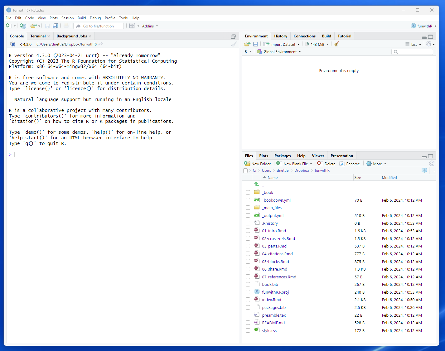
The critical parts for today are the console (the big window on the left) and the environment window (the window at the top right). In each of the areas of the RStudio screen, you can toggle between different things to view, using the tabs (for example, between the Console and the Terminal in the left-hand window, or the Environment and History in the top right-hand window). You will need to look at the console and the environment windows today.
In what follows, R code will appear in grey boxes.
2.3.2 Is anybody in? First interactions with R
Go to the console and click. The cursor after the > symbol will start to blink. You can now type input into the console. Anything you type now will be sent to R as soon as you hit return. For example, do some simple arithmetic:
## [1] 5Yes, you can use R to successfully add 2 and 3 to get five. Try a few others (I have hidden R’s answers):
Perhaps you did not know this last one: 2 ** 3 means 2 to the power of 3.
2.3.3 Objects
R would be of little interest if you could just use it as a calculator. In fact what you are going to do with R is to define objects and then apply functions to those objects. Let’s start with the simplest possible object. Type the following:
What happens? You should see that an object appears in your environment. The environment window conveniently tells you that you have an object called x, and its current value is 3. You have assigned the value 3 to the object ‘x’. The object will remain in the environment for the rest of your R session, allowing you to address it, assign it a different value, delete it or whatever.
By the way, you can also achieve the same result with:
This works fine and does the same thing. However, for reasons to do with clarity and the history of R, assigning is usually done with <-. The symbol ‘=’ is used in calling functions, as we shall see, and, as a double form ‘==’ in logical statements.
So, what can you do with your first, beautiful object? Well, you can perform numerical operations on it:
## [1] 9## [1] 243Who knew that 3 to the power of 5 was 243?
Note that when we performed the operations above (multiplying x by 3 or raising it to the power of 5), the value of x did not change’. If you look at the value of x in your environment window, it should still be 3. You merely printed the result of a computation involving x to the console.
What do we do if we want to change the value of the object instead? To do this, we need to reassign the new value to x:
Read this as: please assign a new value to x, equal to the old value of x multiplied by 3. The x on the left hand side represents the new, post-reassignment value of x; whereas the one on the right hand side represents the current one.
By the way, you can also use exactly the same formulation to make a second object that is derived from the first:
This should create a second object in your environment, y, which is the current value of x, raised to the power of 5. Note that if you now change the value of x, the value of y will not update unless you rerun y <- x ** 5 after changing the value of x. This means that the order you do things in always matters in programming. A computation on an object will depend on the value of that object at that point in the programme, and not its value earlier or later on. For example, the two sequences of code below produce different results, as you can quickly verify by typing the lines yourself.
## [1] 33## [1] 392.3.4 Vectors as objects
R objects can be all kinds of things: individual numbers, bits of text, lists of things, statistical models, data sets, even graphics. But the most fundamental type of object you will work with in R is a vector. A vector is an ordered sequence of numbers or characters. For example, let’s say you have collected some data on people’s scores on a questionnaire. Your five respondents scored 3, 7, 15, 1, and 5 respectively. Let’s input this data into our R session.
Now you should have a new object in your environment, called scores (c(...) means combine). scores is a num object, which means it is a vector of numbers. And [1:5] means that it has five positions in it, each of which is occupied by one of the scores from the participant. If you ask R to print the object, it will print all five entries. You can also use the square brackets to address specific positions within it.
## [1] 3 7 15 1 5## [1] 15## [1] 15 1 5You can perform numeric options on a vector object, and these will be applied to each element of the vector in turn. So:
## [1] 4 8 16 2 6## [1] 6 14 30 2 10Note, again, that this last example does not change the value of the entries in scores. To do that would require scores <- scores *2 (don’t do this now).
2.3.5 Applying functions to objects
All the objects in the world would be no use without being able apply functions to them. Functions are operations we perform on the information in an object, and in R they are always followed with the round brackets (). In fact, you have already encountered a function, c(), in the line scores <- c(3, 7, 15, 1, 5). The objects within the round brackets of a function are called its arguments. The arguments of a function can be individual values, vectors, or other objects, depending on the function in question. Many functions take several arguments.
Let’s apply some other simple functions. Try the following functions yourself and guess what they do:
These are the kinds of functions we are often going to use in statistical analysis.
2.3.6 Classes
Objects in R belong to classes. We have already seen one, the class numeric, which our vector scores belongs to. There are many other classes of object in R: character vectors, factors (this is a special type of ordered character vector), data sets, statistical models, images, lists. We will meet these different classes as we go on.
If you ever want to know what class an object belongs to, use the class() function.
## [1] "numeric"## [1] "character"You can also coerce the class of an object to be something different to what it currently is. For example, there is a class called integer which as you might guess contains only integers. Let’s define a vector of non-integer numbers:
Now let us coerce this object to have the class integer:
## [1] 4 4 5 5 2You see that the entries of v are now coerced to the nearest integer.
2.3.7 Assigning and logical checking
Sometimes we want to establish whether a logical condition is true. For example, we might want to know whether the second element of the vector scores is equal to 7. If we say scores[2] = 7, we will assign the value 11 to the second element of scores, which is what we wanted to do. We wanted to establish whether that is the current value.
When we want to ask the question “R, is the second entry of scores 7?”, we use the double equals sign. This means “check whether this condition is met”, rather than “make it the case that this condition is met”. Try the following:
You should get the answer TRUE. Yes, the second entry in scores is equal to 7. You can also ask the same question for all of the vector scores.
## [1] FALSE TRUE FALSE FALSE FALSEOnly the second entry of scores is 7. For the other entries, the equality is false. A sequence of TRUEs and FALSEs is a special type of object of class logical. Try the following:
## [1] "logical"Make sure you are clear what the first line in the chunk above is doing. The brackets are only there to help you understand; it would work just the same without them.
One of the reasons it is good to use <- for assigning in R, rather than =, is to avoid any possible confusion with logical checking ==.
2.4 Installing and activating a contributed package
Contributed packages define extra functions, and sometimes new types of objects too, to allow you to do specific statistical or data manipulation tasks efficiently and elegantly. A package we are going to use in every week of this course is called tidyverse. Tidyverse is the mother of all packages (it is actually a package consisting of multiple packages). It allows you to load, sort, manipulate, and graph your data.
If you want to use a dishwasher, you first have to install it (bring it to your house and connect it to the water and electricity), and then start it. You install it only once, but you start it every time you want to use it. Likewise with contributed packages. Just once for each computer you use, you need to run the following command. This will download the package and save it locally.
Do this now. You will get a lot of output messages, but hopefully the result will be success.
Then, in every R session where you want to use the package, you need to activate it:
Tidyverse and the functions it contains are now available for use in the current session.
2.5 Scripts
So far, we typed commands straight into the R console. This is not how you would ever actually work with R. Instead, you will perform your data analysis by writing scripts. Scripts are text files that contain multiple lines of R sometimes hundreds or thousands of lines, in order. When you run the script, each line is passed to R for execution, in the order in which they appear in the script.
Opening a script, or starting a new one, works exactly like opening a new document in a Word processing programme. In RStudio, go to File > New > R Script for a new script, or File > Open File for an existing one. You can also use the little icons in the top of the RStudio window. Open a new script now. It should appear in the upper part of the left hand window of RStudio.
The first thing we are going to do with our new script is save it. This raises the question: which directory will it save to? Files are by default saved and looked for in the current working directory. To find out what your current directory is, use the following function:
## [1] "C:/Users/danie/Dropbox/Cogmaster course/bookdown"To set it to something else, you have two choices. You can use the following function and provide the path you want to be the working directory.
Alternatively, in the menu, choose Session > Set Working Directory > Choose Directory and navigate to the directory you wish to use.
Now, set a convenient working directory where you wish to have all your materials from this course. Save your blank script (which is currently called Untitled1, probably) using the menus or icons at the top of the screen. Call it ‘firstscript.R’, or whatever you wish, respecting the .R suffix.
Now, type the following lines into your script, separating them with a return:
paste() is a function that sticks two objects together to make a longer object, in this case, the vector consisting of the text “The product is:”, and a number. Now, run the script by clicking the little Source button at the top right of the script. The output of the script will now appear at the console. You can also source your script using Ctrl + Shift + S. You can run individual lines or sections of the script by placing the cursor on the desired line, or selecting multiple lines, and then using Ctrl + Enter.
What is the point of scripts? A script allows you to write down all the operations involved in your data analysis, in order, so that you can get it perfect and then run it. You can also save it and come back to it tomorrow, send it to your collaborators, and most importantly, publish it with your paper so that anyone can see and reproduce the exact analysis operations that underlie your claims about your results.
A useful feature of scripts is that you can comment them, using the # symbol. A comment line will not be evaluated by R. It is just there for you to leave notes for yourself and for your collaborators and readers.
# First specify two numbers
x <- 5
y <- 3
# Then make a sentence saying what their product is
output <- paste("The product is:", x*y)
# Then print this sentence to the console
print(output)
This does exactly the same thing as the version without comments above, but helps the reader see what is going on.
At the end of the session, always save the latest version of your script. If there are unsaved modifications in it, its name will be in red at the top of the tab.
2.6 Reading in data
There is one more thing to do in this session, which is to learn how to read data into R. We are going to download the raw data from a recently published paper (Fan, Tybur, and Jones 2022). The data are available on the Open Science Framework (OSF) website. We will be learning more about the OSF elsewhere in the course. We are not actually going to do anything with the particular dataset. It is just any old cognitive science dataset to help you understand how to load in data.
First, go to the OSF project associated with the paper (https://osf.io/t476f/). You can also find that URL in the published paper, in the section Open practices of data and code availability. Now, in Files navigate to Stage 2 > Raw Data and download the file GB.csv. You want to download it into your R session’s working directory. Remember, you can see what your working directory is in R by typing:
You can also change it using the menu Session > Set Working Directory or the command setwd().
2.6.1 .csv or .Rdata?
The file you downloaded is in the .csv format. This is the most common format for exchanging raw data, because it is neutral and economical. It just consists of the data values separated by commas (csv stands for comma separated values). Sending data in the .csv format makes no assumptions about what software the recipient might use to process or view it: any spreadsheet or statistical package can handle .csv files. When you publish your raw data, you should probably do so as .csv to maximize accessibility.
There is a downside to using the .csv format: it loses a bunch of information in R objects (for example, if the levels of a variable have a specific logical order, or a column of numbers should actually be considered as text.) To retain that kind of information, as well as have a more flexible file format that can also store statistical results, figures etc., you need to use R’s native file format .Rdata. We will deal with saving and loading .Rdata files elsewhere. Most of the data you load in will probably come as .csv files.
2.6.2 Loading in the data
Open a new script, and head it with:
Remember we are going to need the tidyverse package every time we use R in this course. Run this line.
Now, as the next line add:
## Rows: 1371 Columns: 62
## ── Column specification ──────────────────────────────────
## Delimiter: ","
## chr  (6): PID, PSex, AgtSex, StmCon, AgtNat, AgtAct
## dbl (56): Ift, Psn, Sim, ConFrq, CC1, CC2, CC3, CC4, C...
##
## ℹ Use `spec()` to retrieve the full column specification for this data.
## ℹ Specify the column types or set `show_col_types = FALSE` to quiet this message.
Run this line. With luck, a new object called d has appeared in your environment. d is a class of object called a data frame (in fact, it is a specific type of data frame called a tibble, but that need not worry us unduly.) A data frame has a number of rows, each of which represents one case, and a number of columns, each of which represents one variable. Here, if you look in the environment window, you should see that d contains 1371 observations (i.e. 1371 rows) of 62 variables (i.e. 62 columns). If you click the little blue arrow next to d in the environment window, you will see more information about the 62 variables. For example, the first one is called PID (it is the participant ID variable), is of the class character and consists of long strings, the second is called Ift and consists of numbers, etc.
The variables are sub-parts of the overall data frame. If you want to pull out a particular one, you can use the $ notation. For example, to see the values of the variable Ift in data frame d, it is just:
You should see the first 1000 of a fascinating sequence of 1371 numbers.
You can also apply functions to a variable in d using the same notation. Try these:
As for the variables that are of class character, they consist of strings of characters rather than numbers. Let’s look at the one called PSex (participant sex).
You should see a great long string of Male and Female. If you ask for the mean of this variable, you should get an error, because it is the wrong class for that (try it). You might want to ask instead how many Male and how many Female entries there are, as follows.
##
## Female   Male
##    692    679
That makes sense.
That’s enough for week 1. We now have enough of the basics to proceed further with data analysis in week 2.