8 Good and bad research practices
8.1 Positive predictive value: the replication crisis revisited
It is time to come back to the replication crisis, the discovery that many published results in cognitive science do not generalize to new samples. This discovery was a shock to the field (though some statisticians and methodologists had understood the likely scale of the problem for years, and warned about it). In essence, the problem arose because people thought that ‘statistical significance’ (having a p-value less than 0.05 or 0.01) meant the finding had positive predictive value. Unfortunately this is not the case.
Positive predictive value is, roughly, the probability of out-of-sample generalization. Say that in a trial I give one group of people ibuprofen, and find that their symptoms of depression reduce. I want to know about the positive predictive value of this effect: if I now get new samples from the human population and give them ibuprofen, will their depressive symptoms reduce too, or was the observation in the first sample a fluke? Positive predictive value is an important desideratum in science: a claim that has perfect positive predictive value is, arguably, knowledge; and science is about converting true claims into knowledge, and eliminating false claims from the set of candidates.
Positive predictive value depends on a number of factors, as follows:
The probability of getting a p-value of that magnitude if the null hypothesis is true (this seems like it must be 1/20 by definition, but if you have more than one go at the test, it can be higher than this, as we shall see below).
The a priori probability of the non-null hypothesis being true. For example, if I do an elaborate test of whether I can, from my office in France, predict a number that will be chosen at random by the President of Mexico, then even if I get p < 0.01, I probably shouldn’t believe I can generalizably read the minds of Central American heads of state. It was probably a fluke, because the result has a 1% chance of happening under the null hypothesis, whereas the non-null hypothesis would require a complete revision of everything we know about physics, biology and psychology, and so is super improbable.
The probability that if the non-null hypothesis is true, I will detect that this is the case. This is known as the statistical power of my test. Given that sample sizes are finite, statistical power is never 100%. Other things being equal, the lower the power, the more likely your ‘significant’ p-value is a fluke, and the lower your positive predictive value.
Reviewing these factors, it is clear that some of the practices that have been common in cognitive science have contributed to keeping positive predictive value quite low. Particularly pernicious practices are known as researcher degrees of freedom, hypothesizing after the results are known and inadequate sample sizes. We will review each of these before turning to how to do things bettter.
8.2 Researcher degrees of freedom
When you fit a statistical model to data, you usually have quite a few choices to make. We already saw in the behavioural inhibition dataset that you could choose to include GRT and Age as covariates, or not. So there are a number of models you could fit (Condition only, Condition and Deprivation Score, Condition, Deprivation Score and Age, and so on). For any one of these, you would be able to convince yourself and probably others that this was the appropriate model to fit. Plus, there are many other choices you could make: to include or exclude data from a participant who was much older than the rest, or whose reaction times were really slow, or who turned up late, and so on. Or you could look in just the men in the sample, or just the women. So, the researcher has many degrees of freedom in determining the analysis strategy.
The problem with this is that each set of choices that the researcher could make is, if the null hypothesis is true, an independent drawing from the distribution of p-values. So, if you run all of the possible versions of the analysis, you will sooner or later stumble on one configuration of the model in which something comes out with a small p-value, or allegedly ‘significant’. The graph below shows how the probability of getting at least one significant result (at p < 0.05) rises with the number of tests you perform (with some simplifying assumptions, such as that the tests you do are independent of one another).
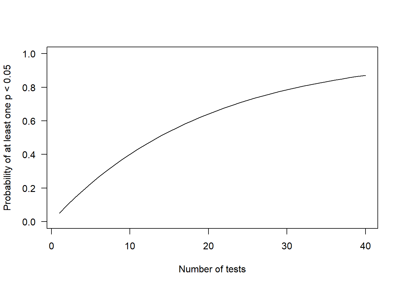
As you can see, if you have a high number of researcher degrees of freedom, and you try out all the options, you will find some significant results. This is particularly pernicious if you then report only some of the specifications that you tried out, specifically the ones that gave you the significant result. The reader will think: oh wow, the first and only thing they tried gives this really small p-value. The reader is not seeing all the other specifications that you tried and rejected. The reader is thus going to infer that the positive predictive value is higher than is really the case.
8.3 Hypothesizing after the results are known (HARKing)
Related to researcher degrees of freedom is hypothesizing after the results are known, or HARKing. In the behavioural inhibition data, for example, there are two reaction times that were measured, the SSRT or stop signal reaction time, and the GRT, the reaction time on the Go trials. Let’s say that I find that Condition affects GRT, with a small p-value, whereas Deprivation Score is associated with SSRT. Of course, I can say, that is exactly what I predicted all along! You would expect being put in a negative mood to slow you down overall, but not specifically affect inhibition, whereas you would expect childhood deprivation to reduce inhibition in particular. And if it is the other way around, Condition affecting SSRT and Deprivation Score affecting GRT, well that makes sense too. Deprivation is going to make all kinds of cognitive performance worse, whereas being in a negative mood specifically reduces inhibition, because you want to do things to escape feeling bad. In other words, whichever way it seems to come out, you can convince others, and definitely yourself, that that is what your hypothesis was anyway.
When HARKing is possible, researchers can perform what are basically exploratory analyses, with many degrees of freedom and many statistical tests, and then present the results as confirmatory results of a single hypothesis. And, guess what, that hypothesis will be supported. Of course it will be, since it has been determined only after the results were known. Cognitive science has a very large prevalence of papers in which hypotheses are supported, which should immediately make us suspicious. Studies where hypotheses are not supported should be common, since most of the plausible hypotheses about the world that humans have entertained over the course of history have turned out not to be true.
8.4 Inadequate sample sizes
On the face of it, the probability of getting a significant p-value is independent of sample size: it is just 1 in 20 for a single test a threshold of p < 0.05, for example. But, given that you have a ‘significant’ p-value, the probability that it is a fluke is in fact higher if your sample size is small and you have fewer observations (Button et al. 2013).
How can this be? Well the probability that the result is a fluke is the probability of getting p < 0.05 if the null hypothesis is true (1 in 20 for a single test), divided by the total probability of getting p < 0.05. And the total probability of getting p < 0.05 is equal to the probability of getting p < 0.05 if the non-null hypothesis is true, multiplied by the prior probability that the non-null hypothesis is true, plus the probability of getting p < 0.05 if the null hypothesis is true. This denominator gets smaller as the probability of getting p < 0.05 if the non-null hypothesis is actually true (the statistical power) gets smaller. And statistical power reduces with the sample size. So, in other words, as your sample size gets smaller, the probability that any p < 0.05 you do come across is a fluke gets bigger, because your ability to detect as significant any real effects gets lower, whereas the probability of flukes is independent of sample size.
In cognitive research, there is no real excuse for inadequate sample sizes, since the experiments are relatively easy to do. But research on babies, or non-human animals, or using neuroscience techniques like brain imaging, is typically massively underpowered, meaning a lot of the ‘significant’ findings in these areas are probably flukes (Button et al. 2013).
8.5 Principles of sound data analysis: PASSAR
Given the replication crisis, how should we produce and analyse data in a way that will make it more likely that the claims we make are true. I recommend you follow the acronym PASSAR:
Predictions are pre-registered.
Analysis plan is pre-registered.
Sample size is adequate and justified.
Sensitivity to analytical decisions is explored.
Available are the data and code for anyone to inspect.
Replication in a different sample has been done where possible.
If all the steps of PASSAR have been followed, then a claim is more plausible than if any one of them is missing. We will now go through them all in turn.
8.5.1 Predictions are pre-registered
The best antidote to hypothesizing after the results are known is being forced to write down your hypotheses and predictions and put them in a locked box before you collect the data. This practice is known as pre-registration. The locked box is metaphorical, of course, it is a third-party website such as the Open Science Framework or OSF (www.osf.io). You post your pre-registration document there and it is date stamped so it is clear when you did this.
We will come to the details of how to write a pre-registration in the next section, but it is a tremendously beneficial exercise for both researcher and reader. For the researcher, it really helps get clear exactly what your hypotheses and predictions were before it is too late. Many is the time that in writing the pre-reg, I have realised that my thinking was muddled or unclear, or that there were two different versions of my hypothesis and I was not sure which one I was interested in. Writing the pre-reg helps you get these things straight, and has improved or aborted many a bad experiment. For the reader, the pre-reg is useful, because it makes completely transparent which things the researcher had genuinely predicted beforehand, and which things were exploratory discoveries. A finding that was predicted beforehand is impressive support for a theory. A finding that was not predicted beforehand but makes a kind of sense in retrospect is less impressive support for a theory. By comparing the pre-reg to the findings, you can tell which is which.
8.5.2 Analysis plan is pre-registered
The analysis plan is the set of steps you intend to carry out to test your predictions. You say what variables you will have or calculate, what statistical models you will fit to those variables, and what parameter estimates or statistical tests you will take to constitute each prediction being supported or not supported. You should enter into as much detail as possible about the kinds of models, as well as their specification, which means which combinations of predictors and covariates they contain. You describe your analysis plan in the same pre-registration document as your predictions.
The primary point of pre-registering the analysis plan is to reduce the researcher’s degrees of freedom. It cuts down (though does not completely eliminate) the thicket of variants of the analysis that the researcher might be tempted to run, and so it reassures the reader that whatever results they are reading really are the output of the first analysis that was run, the one the researcher initially had in mind, and not the outcome of playing with the specification for hours until some p-value came out significant (this pastime is known as p-hacking).
However, pre-registering the analysis plan has a massive secondary benefit. It really speeds up the researcher’s work. Prior to pre-registration, it was not uncommon to finish a study and then say ‘whew! now we have to figure out how you would analyse data like this!’. The process of figuring this out could be very lengthy and often reveal substantial confusion and frustration (turns out, we did not really measure the right things). Making your analysis plan ahead of time really helps you do better science, faster.
In the best case scenario, you can actually write your analysis script before collecting the data, basing it on some pilot data, or on simulated data (we will learn how to simulate data in a later week). Then, when you have the data, the data analysis is very quick, and you soon know what you have found.
Having said all this, you do often need to depart from your pre-registered analysis plan in all kinds of ways. A variable turns out to have a very different distribution from anticipated; or two variables turn out to be highly correlated, necessitating a change of specification. It is because of possibilities like this that you first do sense checking, descriptive statistics, and simple plots (week 2). It’s fine to depart from your pre-registered analysis plan, but where you have done so, your paper or thesis must say that you did, and justify why. ‘We realised that what we had pre-registered wasn’t right’ is a legitimate justification; I myself have used it before! Good science is about being transparent, not omnipotent.
As well as being pre-registered, your analysis plan needs to be a good one! A good analysis plan is what I call trim. A trim analysis is one where the number of models fitted and statistical tests performed is kept to a minimum, so that results are clearly interpretable and p-values are meaningful. We will come to the principles of a trim analysis plan in a later week.
8.5.3 Sample size is adequate and justified
In an ideal study, you would want to be really convinced that a parameter estimate whose confidence interval crossed zero really represented a parameter in the population that is close to zero. That is, a null result should be convincingly null. On the other hand, when you do have a non-zero parameter estimate, you would want to be convinced that it is something more than a fluke. To achieve both of these goals, the sample size needs to be big enough, and the pre-registration and paper need to contain a sample size justification, a reasoned paragraph that explains why whatever the target sample is is big enough to do the job.
Sample size justification usually involves some kind of power analysis (Giner-Sorolla et al. 2024). This refers to a calculation of either how large a sample is needed to detect a true effect of a certain size with a specified probability; or of how large an effect could be detected with a certain probability given a sample size. There are contributed R packages for power analysis covering common situations (such as pwr). Another approach I recommend is to use R to simulate the data you might collect. By simulating multiple times under different assumptions about effect size and sample size, you will be able to see how often you detect a significant result. We will learn how to simulate datasets in a subsequent week.
8.5.4 Sensitivity to analytical decisions is explored
Even if you pre-registered your analysis plan, there are probably decisions you had to make about the exact specification of your model; decisions that you could have made differently. There are almost always several possible reasonable analyses to answer a given question.
In these circumstances, one wants to know: is the significant (or null) result that you are reporting found only in the particular specification that you chose, or in all of the reasonable specifications that you might have come up; or somewhere in between. It is good to explore and report the extent to which your conclusions are sensitive to analytical decisions you made (for example about transformation of the outcome variable, inclusion of covariates, and so on).
An informal way of performing sensitivity analysis is to perform the most obvious alternative analysis (for example, one you thought about and dismissed). You can then mention that you did this and whether it affected the conclusion. In the behavioural inhibition paper, the researchers examined whether log-transforming SSRT versus not doing so made any difference to their conclusion, and reported that it did not.
A more formal and elaborate way of exploring sensitivity to analytical decisions is multiverse analysis or specification curve analysis. In these techniques, you list all the possible statistical models that you might have thought reasonable to answer the question, and you fit all of them. You get a range of parameter estimates, and a range of p-values. This allows you to say something like: our preferred analysis gives us a parameter estimate of 0.5, and the whole set of possible analyses that might reasonably have been performed produce parameter estimates between 0.1 and 0.7, with a mean of 0.4 (or whatever). You can also explore which features of the specification lead to higher and lower parameter estimates (maybe, in the behavioural inhibition example, including GRT as a covariate tends to reduce the parameter estimate for Deprivation Score, or whatever,.
When you report your results, a section exploring sensitivity to analytical decisions is always a good inclusion, whether that be a full report of alternative results; a supplement or appendix; or just a brief mention in the text.
8.5.5 Available are the data and code for anyone to inspect.
When you submit your paper or thesus, it is imperative that your raw data and your analysis code are posted in a repository that anyone can access, like the Open Science Framework. There should be a clear link in the document to where the data and code can be found.
There are several reasons for doing this. First, you are making scientific claims, and you need to make transparent the evidential grounds for those claims. Your paper or thesis will give only a compressed description of the information you have gathered. You won’t report every analytical nuance or every descriptive aspect of the dataset in the text. People need to be able to look for themselves to assess whether what you are saying is really supported, or whether there might be alternative analyses that lead to a different conclusion.
Second, your data might be useful for answering a different question than the one you thought of. The behavioural inhibition data were intended for answering questions about effects of socioeconomic deprivation and mood, but they could be useful for someone who wants to understand whether there are gender differences in reaction time. People who perform meta-analyses are always looking out for existing data that can be used to address a specific question. By posting the data online, you contribute to the collective endeavour of science.
Third, archiving the data and code properly online is really useful for you. You might come back to your research project a year or five years or ten years later. If the data and code have been put onto the repository in a really clear and well-organized way, this will be easy. If not, you will be looking around on the hard drive of an old computer trying desperately to work out which is the right version. The person who is most helped by proper archiving (as for pre-registration) is future you.
Good practices for useful archiving of data and code are:
Anonymizing data to avoid identifying your participants. Obviously this means removing names, addresses and emails, but potentially also other things like geographic location, IP address or other revealing information;
Having sensible variable names, not
bb40butgender, and so on;For qualitative variables, coding them with transparent words (
negativeandneutal, not1and2);If your dataset contains many variables or is complicated, providing a codebook that explains what each variable is and how it is derived or coded;
Sub-dividing your scripts if necessary. For example, for some complex projects, I provide the data in their rawest form, plus two scripts: a data processing script that makes the raw data into a usable dataframe for analysis, and then an analysis script that exactly reproduces everything reported in the paper. This way everything is reproducible, but a lot of the behind-the-scenes recoding and merging is relegated to a preliminary script that just needs to be run once;
Commenting your scripts really well (use # for a comment remember). This includes saying what each section is aiming to do (load in the data, fit a model, make the figures, etc.), as well as comments every few lines that relate to specific function calls or operations. Commenting is incredibly helpful and people generally don’t do enough. It helps your collaborators and future you as well!
8.5.6 Replication
Given that many statistically significant results are flukes, it is essential that any significant result be replicated. Until it has been replicated, it barely has the status of a claim. Historically, cognitive science has done an inefficiently small amount of replication. This is because it was considered cooler and more important to find out novel things. But, it has the unfortunate consequence that the list of novel published findings that probably aren’t true gets longer and longer, and we don’t make any actual progress identifying knowledge.
Replication can be internal (done by the same researchers) or external (done by someone else). These days, a cognitive science paper really ought to have at least one internal replication. That is, if you have an experiment that produced a result, then do the experiment again in a new sample and report that alongside the first one. You can do it again unchanged, or add some extension as long as doing so does not undermine the basic function of replication. Before your claims count as well supported, there will need to be external replication (done by someone else) as well. Obviously, that is beyond your control. The best you can do is get your study and data out there and hope that it interests someone to replicate it.
Replication can be exact (that is, doing the very same procedure with a novel sample), or generalizing (that is, doing the study in a slightly different way or different population or using different measures of the same construct). The two kinds of replication have different functions. Exact replication is the critical first step, to show that the finding is not just chance. Generalizing replication (of many kinds) must then follow, to show that the general conclusion is not critically dependent on testing in a certain population, with a certain set of stimuli, or a certain way of measuring the outcome. You should start off with exact replication before considering if some kind of generalizing replication is possible within the constraints of your project.
8.6 Writing a pre-registration
We will conclude this week by looking at how to write a pre-registration. There are a number of different templates for pre-registrations available, and you can just write your own document using whatever structure you find useful.
The rest of this sectionnreproduces a set of recommended headings and sections for pre-registrations provided by the Open Science Framework (see https://osf.io/preprints/metaarxiv/epgjd). Note that the OSF occasionally uses different terminology or uses the same terminology differently than I have done so far. There are also some terms we have not covered in this course; don’t worry about these. The pre-registration structure works better for some studies than others. In some cases, you may just have to put ‘not applicable’ for certain sections.
8.6.1 Study Information
8.6.1.1 Title
Provide the working title of your study. It may be the same title that you submit for publication of your final manuscript, but it is not a requirement.
Example: Effect of sugar on brownie tastiness.
More info: The title should be a specific and informative description of a project. Vague titles such as ‘Fruit fly preregistration plan’ are not appropriate.
8.6.1.3 Description
Please give a brief description of your study, including some background, the purpose of the of the study, or broad research questions.
Example: Though there is strong evidence to suggest that sugar affects taste preferences, the effect has never been demonstrated in brownies. Therefore, we will measure taste preference for four different levels of sugar concentration in a standard brownie recipe to determine if the effect exists in this pastry.
More info: The description should be no longer than the length of an abstract. It can give some context for the proposed study, but great detail is not needed here for your preregistration.
8.6.1.4 Hypotheses
List specific, concise, and testable hypotheses. Please state if the hypotheses are directional or non-directional. If directional, state the direction. A predicted effect is also appropriate here. If a specific interaction or moderation is important to your research, you can list that as a separate hypothesis.
Example: If taste affects preference, then mean preference indices will be higher with higher concentrations of sugar.
8.6.2 Design Plan
In this section, you will be asked to describe the overall design of your study. Remember that this research plan is designed to register a single study, so if you have multiple experimental designs, please complete a separate preregistration.
8.6.2.1 Study Type
- Experiment - A researcher randomly assigns treatments to study subjects, this includes field or lab experiments. This is also known as an intervention experiment and includes randomized controlled trials.
- Observational Study - Data is collected from study subjects that are not randomly assigned to a treatment. This includes surveys, ñnatural experiments,î and regression discontinuity designs.
- Meta-Analysis - A systematic review of published studies.
- Other (explain your study type)
8.6.2.2 Blinding
Blinding describes who is aware of the experimental manipulations within a study. Delete all that do not apply.
- No blinding is involved in this study.
- For studies that involve human subjects, they will not know the treatment group to which they have been assigned.
- Personnel who interact directly with the study subjects (either human or non-human subjects) will not be aware of the assigned treatments. (Commonly known as “double blind”).
- Personnel who analyze the data collected from the study are not aware of the treatment applied to any given group.
8.6.2.3 Is there any additional blinding in this study?
Describe any additional blinding procedures that were not covered by the options above.
8.6.2.4 Study design
Describe your study design. Examples include two-group, factorial, randomized block, and repeated measures. Is it a between (unpaired), within-subject (paired), or mixed design? Describe any counterbalancing required. Typical study designs for observation studies include cohort, cross sectional, and case-control studies.
Example: We have a between subjects design with 1 factor (sugar by mass) with 4 levels.
More info: This question has a variety of possible answers. The key is for a researcher to be as detailed as is necessary given the specifics of their design. Be careful to determine if every parameter has been specified in the description of the study design. There may be some overlap between this question and the following questions. That is OK, as long as sufficient detail is given in one of the areas to provide all of the requested information. For example, if the study design describes a complete factorial, 2 X 3 design and the treatments and levels are specified previously, you do not have to repeat that information.
8.6.2.5 Randomization
If you are doing a randomized study, how will you randomize, and at what level?
Example: We will use block randomization, where each participant will be randomly assigned to one of the four equally sized, predetermined blocks. The random number list used to create these four blocks will be created using the web applications available at http://random.org.
More info: Typical randomization techniques include: simple, block, stratified, and adaptive covariate randomization. If randomization is required for the study, the method should be specified here, not simply the source of random numbers.
8.6.3 Sampling Plan
In this section we’ll ask you to describe how you plan to collect samples, as well as the number of samples you plan to collect and your rationale for this decision. Please keep in mind that the data described in this section should be the actual data used for analysis, so if you are using a subset of a larger dataset, please describe the subset that will actually be used in your study.
8.6.3.1 Existing data
Preregistration is designed to make clear the distinction between confirmatory tests, specified prior to seeing the data, and exploratory analyses conducted after observing the data. Therefore, creating a research plan in which existing data will be used presents unique challenges. Please select the description that best describes your situation. Please do not hesitate to contact the COS if you have questions about how to answer this question (prereg@cos.io).
Delete all that do not apply.
- Registration prior to creation of data: As of the date of submission of this research plan for preregistration, the data have not yet been collected, created, or realized.
- Registration prior to any human observation of the data: As of the date of submission, the data exist but have not yet been quantified, constructed, observed, or reported by anyone - including individuals that are not associated with the proposed study. Examples include museum specimens that have not been measured and data that have been collected by non-human collectors and are inaccessible.
- Registration prior to accessing the data: As of the date of submission, the data exist, but have not been accessed by you or your collaborators. Commonly, this includes data that has been collected by another researcher or institution.
- Registration prior to analysis of the data: As of the date of submission, the data exist and you have accessed it, though no analysis has been conducted related to the research plan (including calculation of summary statistics). A common situation for this scenario when a large dataset exists that is used for many different studies over time, or when a data set is randomly split into a sample for exploratory analyses, and the other section of data is reserved for later confirmatory data analysis.
- Registration following analysis of the data: As of the date of submission, you have accessed and analyzed some of the data relevant to the research plan. This includes preliminary analysis of variables, calculation of descriptive statistics, and observation of data distributions. Please see cos.io/prereg for more information.
8.6.3.2 Explanation of existing data
If you indicate that you will be using some data that already exist in this study, please describe the steps you have taken to assure that you are unaware of any patterns or summary statistics in the data. This may include an explanation of how access to the data has been limited, who has observed the data, or how you have avoided observing any analysis of the specific data you will use in your study.
Example: An appropriate instance of using existing data would be collecting a sample size much larger than is required for the study, using a small portion of it to conduct exploratory analysis, and then registering one particular analysis that showed promising results. After registration, conduct the specified analysis on that part of the dataset that had not been investigated by the researcher up to that point.
More info: An appropriate instance of using existing data would be collecting a sample size much larger than is required for the study, using a small portion of it to conduct exploratory analysis, and then registering one particular analysis that showed promising results. After registration, conduct the specified analysis on that part of the dataset that had not been investigated by the researcher up to that point.
8.6.3.3 Data collection procedures
Please describe the process by which you will collect your data. If you are using human subjects, this should include the population from which you obtain subjects, recruitment efforts, payment for participation, how subjects will be selected for eligibility from the initial pool (e.g. inclusion and exclusion rules), and your study timeline. For studies that donÍt include human subjects, include information about how you will collect samples, duration of data gathering efforts, source or location of samples, or batch numbers you will use.
Example: Participants will be recruited through advertisements at local pastry shops. Participants will be paid $10 for agreeing to participate (raised to $30 if our sample size is not reached within 15 days of beginning recruitment). Participants must be at least 18 years old and be able to eat the ingredients of the pastries.
More information: The answer to this question requires a specific set of instructions so that another person could repeat the data collection procedures and recreate the study population. Alternatively, if the study population would be unable to be reproduced because it relies on a specific set of circumstances unlikely to be recreated (e.g., a community of people from a specific time and location), the criteria and methods for creating the group and the rationale for this unique set of subjects should be clear.
8.6.3.4 Sample size
Describe the sample size of your study. How many units will be analyzed in the study? This could be the number of people, birds, classrooms, plots, interactions, or countries included. If the units are not individuals, then describe the size requirements for each unit. If you are using a clustered or multilevel design, how many units are you collecting at each level of the analysis?
Example: Our target sample size is 280 participants. We will attempt to recruit up to 320, assuming that not all will complete the total task.
More information: For some studies, this will simply be the number of samples or the number of clusters. For others, this could be an expected range, minimum, or maximum number.
8.6.3.5 Sample size rationale
This could include a power analysis or an arbitrary constraint such as time, money, or personnel.
Example: We used the software program G*Power to conduct a power analysis. Our goal was to obtain .95 power to detect a medium effect size of .25 at the standard .05 alpha error probability.
More information: This gives you an opportunity to specifically state how the sample size will be determined. A wide range of possible answers is acceptable; remember that transparency is more important than principled justifications. If you state any reason for a sample size upfront, it is better than stating no reason and leaving the reader to “fill in the blanks.” Acceptable rationales include: a power analysis, an arbitrary number of subjects, or a number based on time or monetary constraints.
8.6.3.6 Stopping rule
If your data collection procedures do not give you full control over your exact sample size, specify how you will decide when to terminate your data collection.
Example: We will post participant sign-up slots by week on the preceding Friday night, with 20 spots posted per week. We will post 20 new slots each week if, on that Friday night, we are below 320 participants.
More information: You may specify a stopping rule based on p-values only in the specific case of sequential analyses with pre-specified checkpoints, alphas levels, and stopping rules. Unacceptable rationales include stopping based on p-values if checkpoints and stopping rules are not specified. If you have control over your sample size, then including a stopping rule is not necessary, though it must be clear in this question or a previous question how an exact sample size is attained.
8.6.4 Variables
In this section you can describe all variables (both manipulated and measured variables) that will later be used in your confirmatory analysis plan. In your analysis plan, you will have the opportunity to describe how each variable will be used. If you have variables which you are measuring for exploratory analyses, you are not required to list them, though you are permitted to do so.
8.6.4.1 Manipulated variables
Describe all variables you plan to manipulate and the levels or treatment arms of each variable. This is not applicable to any observational study.
Example: We manipulated the percentage of sugar by mass added to brownies. The four levels of this categorical variable are: 15%, 20%, 25%, or 40% cane sugar by mass.
More information: For any experimental manipulation, you should give a precise definition of each manipulated variable. This must include a precise description of the levels at which each variable will be set, or a specific definition for each categorical treatment. For example, “loud or quiet,” should instead give either a precise decibel level or a means of recreating each level. ‘Presence/absence’ or ‘positive/negative’ is an acceptable description if the variable is precisely described.
8.6.4.2 Measured variables
Describe each variable that you will measure. This will include outcome measures, as well as any predictors or covariates that you will measure. You do not need to include any variables that you plan on collecting if they are not going to be included in the confirmatory analyses of this study.
Example: The single outcome variable will be the perceived tastiness of the single brownie each participant will eat. We will measure this by asking participants ‘How much did you enjoy eating the brownie’ (on a scale of 1-7, 1 being ‘not at all’, 7 being ‘a great deal’) and ‘How good did the brownie taste’ (on a scale of 1-7, 1 being ‘very bad’, 7 being ‘very good’).
More information: Observational studies and meta-analyses will include only measured variables. As with the previous questions, the answers here must be precise. For example, ‘intelligence,’ ‘accuracy,’ ‘aggression,’ and ‘color’ are too vague. Acceptable alternatives could be ‘IQ as measured by Wechsler Adult Intelligence Scale’ ‘percent correct,’ ‘number of threat displays,’ and ‘percent reflectance at 400 nm.’
8.6.4.3 Indices
If any measurements are going to be combined into an index (or even a mean), what measures will you use and how will they be combined? Include either a formula or a precise description of your method. If your are using a more complicated statistical method to combine measures (e.g. a factor analysis), you can note that here but describe the exact method in the analysis plan section.
Example: We will take the mean of the two questions above to create a single measure of ‘brownie enjoyment.’
More information: If you are using multiple pieces of data to construct a single variable, how will this occur? Both the data that are included and the formula or weights for each measure must be specified. Standard summary statistics, such as “means” do not require a formula, though more complicated indices require either the exact formula or, if it is an established index in the field, the index must be unambiguously defined. For example, “biodiversity index” is too broad, whereas “Shannon’s biodiversity index” is appropriate.
8.6.5 Analysis Plan
You may describe one or more confirmatory analysis in this preregistration. Please remember that all analyses specified below must be reported in the final article, and any additional analyses must be noted as exploratory or hypothesis generating.
A confirmatory analysis plan must state up front which variables are predictors (independent) and which are the outcomes (dependent), otherwise it is an exploratory analysis. You are allowed to describe any exploratory work here, but a clear confirmatory analysis is required.
8.6.5.1 Statistical models
What statistical model will you use to test each hypothesis? Please include the type of model (e.g. ANOVA, multiple regression, SEM, etc) and the specification of the model (this includes each variable that will be included as predictors, outcomes, or covariates). Please specify any interactions, subgroup analyses, pairwise or complex contrasts, or follow-up tests from omnibus tests. If you plan on using any positive controls, negative controls, or manipulation checks you may mention that here. Remember that any test not included here must be noted as an exploratory test in your final article.
Example: We will use a one-way between subjects ANOVA to analyze our results. The manipulated, categorical independent variable is ‘sugar’ whereas the dependent variable is our taste index.
More information: This is perhaps the most important and most complicated question within the preregistration. As with all of the other questions, the key is to provide a specific recipe for analyzing the collected data. Ask yourself: is enough detail provided to run the same analysis again with the information provided by the user? Be aware for instances where the statistical models appear specific, but actually leave openings for the precise test. See the following examples:
If someone specifies a 2x3 ANOVA with both factors within subjects, there is still flexibility with the various types of ANOVAs that could be run. Either a repeated measures ANOVA (RMANOVA) or a multivariate ANOVA (MANOVA) could be used for that design, which are two different tests. If you are going to perform a sequential analysis and check after 50, 100, and 150 samples, you must also specify the p-values you’ll test against at those three points.
8.6.5.2 Transformations
If you plan on transforming, centering, recoding the data, or will require a coding scheme for categorical variables, please describe that process.
Example: The “Effect of sugar on brownie tastiness” does not require any additional transformations. However, if it were using a regression analysis and each level of sweet had been categorically described (e.g. not sweet, somewhat sweet, sweet, and very sweet), ‘sweet’ could be dummy coded with ‘not sweet’ as the reference category.
More information: If any categorical predictors are included in a regression, indicate how those variables will be coded (e.g. dummy coding, summation coding, etc.) and what the reference category will be.
8.6.5.3 Inference criteria
What criteria will you use to make inferences? Please describe the information you’ll use (e.g. p-values, bayes factors, specific model fit indices), as well as cut-off criterion, where appropriate. Will you be using one or two tailed tests for each of your analyses? If you are comparing multiple conditions or testing multiple hypotheses, will you account for this?
Example: We will use the standard p<.05 criteria for determining if the ANOVA and the post hoc test suggest that the results are significantly different from those expected if the null hypothesis were correct. The post-hoc Tukey-Kramer test adjusts for multiple comparisons.
More information: P-values, confidence intervals, and effect sizes are standard means for making an inference, and any level is acceptable, though some criteria must be specified in this or previous fields. Bayesian analyses should specify a Bayes factor or a credible interval. If you are selecting models, then how will you determine the relative quality of each? In regards to multiple comparisons, this is a question with few “wrong” answers. In other words, transparency is more important than any specific method of controlling the false discovery rate or false error rate. One may state an intention to report all tests conducted or one may conduct a specific correction procedure; either strategy is acceptable.
8.6.5.4 Data exclusion
How will you determine what data or samples, if any, to exclude from your analyses? How will outliers be handled? Will you use any awareness check?
Example: No checks will be performed to determine eligibility for inclusion besides verification that each subject answered each of the three tastiness indices. Outliers will be included in the analysis.
More information: Any rule for excluding a particular set of data is acceptable. One may describe rules for excluding a participant or for identifying outlier data.
8.6.5.5 Missing data
How will you deal with incomplete or missing data?
Example: If a subject does not complete any of the three indices of tastiness, that subject will not be included in the analysis.
More information: Any relevant explanation is acceptable. As a final reminder, remember that the final analysis must follow the specified plan, and deviations must be either strongly justified or included as a separate, exploratory analysis.
8.6.5.6 Exploratory analysis
If you plan to explore your data set to look for unexpected differences or relationships, you may describe those tests here. An exploratory test is any test where a prediction is not made up front, or there are multiple possible tests that you are going to use. A statistically significant finding in an exploratory test is a great way to form a new confirmatory hypothesis, which could be registered at a later time.
Example: We expect that certain demographic traits may be related to taste preferences. Therefore, we will look for relationships between demographic variables (age, gender, income, and marital status) and the primary outcome measures of taste preferences.
8.6.6 Other
8.6.6.1 Other
If there is any additional information that you feel needs to be included in your preregistration, please enter it here. Literature cited, disclosures of any related work such as replications or work that uses the same data, or other context that will be helpful for future readers would be appropriate here.
Enter any additional information not covered by other sections, or state not applicable.
8.7 Summary
In this session, we have:
Revisited the practices that lead to a low positive predictive value in cognitive science findings, including researcher degrees of freedom, hypothesizing after the results are known, and inadequate sample size;
Introduced the PASSAR acronym for principles of good data production and analysis;
Examined what a pre-registration looks like through the Open Science Framework template.