10 Models with interactions
10.1 Introduction
This session extends our use of the General Linear Model to the where there are not just several predictor variables, but you want to allow for interactions we will explain the idea of an interaction as we go but, in essence, this refers to the possibility that you can’t adequately describe how one predictor variable affects the outcome without referring to the level of another predictor variable.
10.2 Reloading the Fitouchi et al. data
Let’s reload the data that we plotted in session 9 (Fitouchi et al. 2022). You might want to refer back to that session to remind yourself what the study was about;
## Rows: 379 Columns: 24
## ── Column specification ──────────────────────────────────
## Delimiter: ","
## chr  (1): Condition
## dbl (23): character_1, character_2, character_3, chara...
##
## ℹ Use `spec()` to retrieve the full column specification for this data.
## ℹ Specify the column types or set `show_col_types = FALSE` to quiet this message.
Now, let’s see a version of that figure 2 that we plotted in session 9, where the change in cooperativeness was plotted against the participant’s puritanism score.
df7 %>%
  ggplot(aes(x=puritanism_score, y=coop_score, colour=Condition)) +
  geom_point() +
  geom_smooth(method="lm", linetype="dotted") +
  theme_classic() +
  xlab("Puritanism score") +
  ylab("Change in cooperativeness") +
  scale_colour_manual(values=c("darkred", "darkgreen"))
## `geom_smooth()` using formula = 'y ~ x'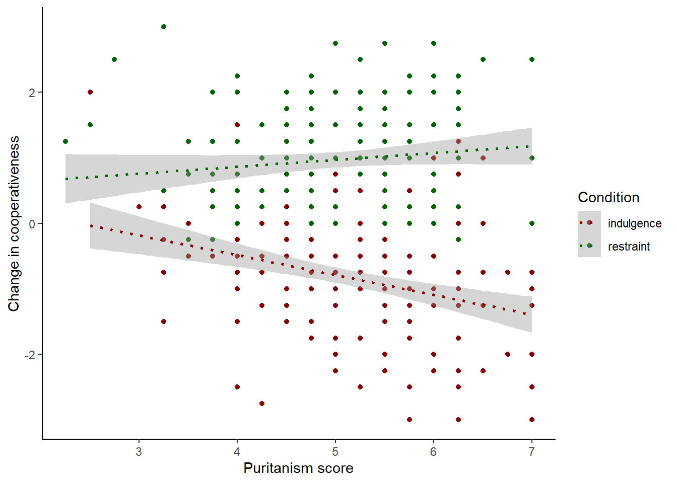
Eyeballing the graph, it looks like there is a relationship between puritanism score and change in cooperativeness, but the nature of that relationship depends on condition. In the indulgence condition, it appears to be a negative relationship, whereas in the restraint condition, it appears to be a positive one.
If we think about the design of the study, this makes sense. The puritanism score variable is a measure of the tendency of the person to hold puritanical attitudes. In the indulgence condition, the participants read that the person in the vignette was indulging in more pleasures. The hypothesis was that they would think he would become less cooperative; and this would be particularly true the more puritanical their attitudes. In the restraint condition, they read that he had cut down on pleasures. The hypothesis was that they would think he would become more cooperative, and again, this would be more strongly true the more puritanical their attitudes. So, the different relationships between puritanism and change in cooperation are expected. You can’t describe the expected relationship between puritanism score and change in cooperation without also knowing which condition it is.
10.3 General Linear models for situations with interactions
10.3.1 Start with an additive model
In a situation with an interaction, there are (at least) two predictor variables that matter. Using what we did in previous sessions, we can quickly set up a General Linear Model with two predictor variables, puritanism_score and Condition, with coop_score as the outcome.
##
## Call:
## lm(formula = coop_score ~ Condition + scale(puritanism_score),
##     data = df7)
##
## Residuals:
##      Min       1Q   Median       3Q      Max
## -2.27106 -0.55983 -0.00364  0.55646  2.54151
##
## Coefficients:
##                         Estimate Std. Error t value
## (Intercept)             -0.80286    0.05980 -13.425
## Conditionrestraint       1.76931    0.08609  20.552
## scale(puritanism_score) -0.09387    0.04308  -2.179
##                         Pr(>|t|)
## (Intercept)               <2e-16 ***
## Conditionrestraint        <2e-16 ***
## scale(puritanism_score)   0.0299 *
## ---
## Signif. codes:
## 0 '***' 0.001 '**' 0.01 '*' 0.05 '.' 0.1 ' ' 1
##
## Residual standard error: 0.837 on 376 degrees of freedom
## Multiple R-squared:  0.534,  Adjusted R-squared:  0.5315
## F-statistic: 215.5 on 2 and 376 DF,  p-value: < 2.2e-16
This appears to show that both Condition and puritanism_score matter for coop_score, with a positive coefficient for Condition (higher coop_score in the restraint condition) and a negative coefficient for puritanism_score (lower coop_score the higher the participant’s puritanism_score). Is this capturing the hypothetical expectation?
The model m1 is not adequate to the task. Let’s look at the implied equation of the model:
\[ E(coop\_score) = \beta_0 + \beta_1 * Condition + \beta_2 * puritanism\_score \]
That is, the predicted value of coop_score for a participant is going to be \(\beta_0\), plus \(\beta_1\) if they are in the restraint condition, plus \(\beta_2\) for every standard deviation higher in puritanism_score they are (remember the \(\beta\) are parameters that the model estimates from the data). However, \(\beta_2\) is mandated to be the same regardless of condition, which means that we assume that an extra standard deviation of puritanism_score is the same in the indulgence condition as in the restraint condition. If we wanted to graph what this model is assuming about the situation, it would look like this:
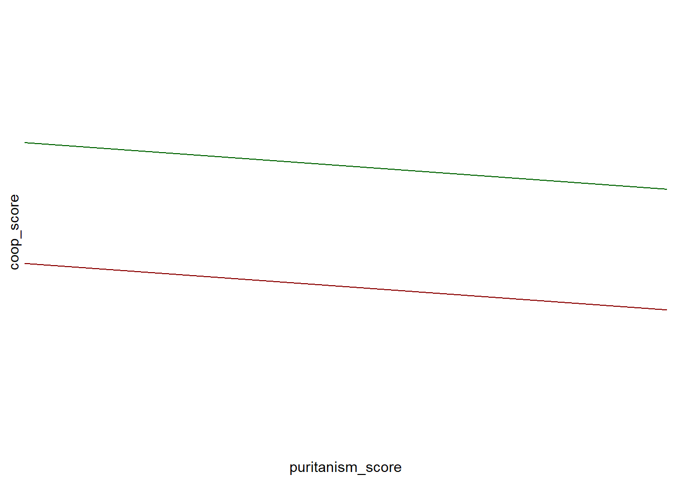
The effects of Condition and puritanism_score are just added together, and for this reason, m1 is known as an additive model. What we want, by contrast, is that the level of Condition modifies the slope of coop_score on puritanism_score. This is called an interactive model.
10.3.2 Specifying and fitting an interactive model
The implied equation of an interactive model looks like this:
\[ E(coop\_score) = \beta_0 + \beta_1 * Condition + \beta_2 * puritanism\_score \\+ \beta_3 * Condition*puritanism\_score \]
Here, the predicted value of someone’s cooperative score would be \(\beta_0\), plus \(\beta_1\) if the condition is restraint, plus \(\beta_2\) for every standard deviation of puritanism_score, plus \(\beta_3\) for every standard deviation of puritanism_score only if the condition is restraint. Thus, the slope of the relationship between coop_score and puritanism_score is \(\beta_2\) in the indulgence condition, and \(\beta_2 + \beta_3\) in the restraint condition. \(\beta_3\) could end up being estimated at zero, meaning that the slopes are the same in the two conditions, and our model becomes equivalent to m1. But it could also end up being estimated at something other than zero, in which case the slopes are different in the two conditions. In this case, we would say that there is an interaction between Condition and puritanism_score.
Let’s fit the interaction model:
m2 <-lm(coop_score ~ Condition + scale(puritanism_score) +
          Condition:scale(puritanism_score), data=df7)
summary(m2)
##
## Call:
## lm(formula = coop_score ~ Condition + scale(puritanism_score) +
## Condition:scale(puritanism_score), data = df7)
##
## Residuals:
## Min 1Q Median 3Q Max
## -2.18913 -0.56827 -0.03773 0.51507 2.41647
##
## Coefficients:
## Estimate
## (Intercept) -0.79656
## Conditionrestraint 1.77007
## scale(puritanism_score) -0.27499
## Conditionrestraint:scale(puritanism_score) 0.37070
## Std. Error
## (Intercept) 0.05841
## Conditionrestraint 0.08406
## scale(puritanism_score) 0.05881
## Conditionrestraint:scale(puritanism_score) 0.08414
## t value
## (Intercept) -13.638
## Conditionrestraint 21.058
## scale(puritanism_score) -4.676
## Conditionrestraint:scale(puritanism_score) 4.406
## Pr(>|t|)
## (Intercept) < 2e-16 ***
## Conditionrestraint < 2e-16 ***
## scale(puritanism_score) 4.09e-06 ***
## Conditionrestraint:scale(puritanism_score) 1.38e-05 ***
## ---
## Signif. codes:
## 0 '***' 0.001 '**' 0.01 '*' 0.05 '.' 0.1 ' ' 1
##
## Residual standard error: 0.8172 on 375 degrees of freedom
## Multiple R-squared: 0.557, Adjusted R-squared: 0.5534
## F-statistic: 157.1 on 3 and 375 DF, p-value: < 2.2e-16This makes sense. The implied slope of coop_score on puritanism_score in the indulgence condition is -0.275 (negative, as expected), whereas the implied slope in the restraint condition is \(-0.275 + 0.371 = 0.096\) which is positive, also as expected.
Note that I scaled puritanism_score. This is particularly recommended in models with interactions as it makes the parameters easy to intepret. In the case, the \(\beta_1\) estimate (1.770) represents the effect of going from the indulgence to the restraint condition when puritanism_score is at its average value, which is an easy quantity to get your head around. If you don’t scale, it would represent the effect of going from the indulgence to the restraint condition when puritanism_score is zero. Since very few people do score zero, this is a less useful quantity.
10.3.3 An alternative way of specifying an interaction model
There is also a shorthand way of specifying our interactive model, as follows:
If you fit this you will see that it is identical to m2. So what is the difference? The * notation means ‘these things and all possible interactions between them’. When there are just two variables, this is the same as what we have already done because there is only one possible interaction between two variables. But, when there are more than two variables, there are many possible interactions (with variables A, B and C, the potential interactions are A:B, A:C, B:C and A:B:C). You might want only some of these in your model as only some are relevant to your hypothesis. Using the full-form specification using the : notation allows you to control which interactions should be included and which ones not.
10.4 When should you fit interactions?
Interactive models allow for the effects of some predictor variables to modify the effects of others. They are in a sense more general than the corresponding additive models. Indeed, the corresponding additive models are just the special case of the interactive models where all the interaction terms are zero. Why not, therefore, always specify your models to include all possible interaction terms?
The problem with this is that interactive models quickly become very complex. The number of possible interaction terms rises exponentially with the number of predictor variables. Other things being equal, simpler models are preferable to more complex ones. The results can also become hard to interpret or to relate to your question if you have many interaction terms.
As a rule of thumb, for observational studies, especially those with many potential predictors, only fit interaction terms where you have some reason to predict them. Otherwise just specify the additive terms.
For experimental studies, there is a tradition of fitting all the interaction terms relating to your independent variables (i.e. your manipulated variables). For covariates, you don’t usually fit any interactions unless you have reason to predict them (as we did in the Fitouchi case). This is however only a rule of thumb and might not always be the best approach. The most important thing is to make sure that the specification of your model relates to your research question and predictions. If the question of interest involves one variable modifying the effect of another, then obviously you need to include the relevant interaction term in the specification of your model. If your prediction was for an interaction, then obviously you have to fit that interaction. You model can only ‘see’ the things in the data that its specification allows for.
10.5 Use interaction models to test for differences in association across levels of another variable
A very important thing to stress is that if you want to make a claim that the effect of one variable is different according to the level of another variable, you must use an interactive model.
People often fail to do this right. Instead they often do the following: they divide their data into subsets based on some grouping variable like gender. They find that, say, their experimental effect is ‘significant’ (p < 0.05) in the women subset and not significant in the men subset. They make some conclusion like ‘this treatment has an effect in women but not in men’.
However, they have not shown that the effect of the treatment is any different in women and in men. If you split your dataset it half, your statistical power to detect an effect will be lower in either of the halves than in the whole dataset. So, if you make a load of subsets, even by random sampling, the effect is going to be ‘significant’ (p < 0.05) in some of the subsets and not others, just by chance. This is true even if the actual underlying effect is consistent across all cases. It may well be the case that your parameter estimate is similar in the women and men subsets (at least, with overlapping confidence intervals), but, the p-value happens to be one side of the significance line in one case and the other side in the other. So finding difference of significance across genders does not mean that you have found significance of difference.
If you want to test the hypothesis that the effect of your treatment is different in women and men, the onlyway of doing this is testing whether the interaction term is significantly different from zero in a model which contains treatment, gender, and the interaction of treatment and gender. Very often you will find that the interaction term is not significantly different from zero (therefore, no evidence of a difference in effect by gender), even if the effect of treatment is significant in one subset of the data and not in the other.
10.6 Summary
In this session, we have examined what an interactive model is, and got a sense of what kinds of situations it is useful for. We learned how to specify interaction terms in General Linear Models in R, and how to interpret the output. We also discussed some rules of thumb for which interaction terms you should include in your models.