17 Metaanalysis
17.1 Introduction
It is often the case in science that we have several studies asking more or less the same question, and, hence, several estimates of some parameter such as the strength of association between two variables, or the causal effect of some intervention on some outcome. At this point, we want to synthesize the evidence available to us to come to a conclusion. What, on the basis of all we know so far, is our best current belief on the topic?
Traditionally, people wrote review articles (often known these days, disparagingly, as ‘narrative reviews’). In these reviews, which were often taken as settling a question, an author wrote some text about a number of related studies, compared and contrasted their findings, and informally came to some kind of conclusion. Individual papers also contained literature review sections that did the same thing in miniature.
This is a terrible way of synthesizing evidence, for a number of reasons. In fact, reliance on narrative reviews by influential people often hindered the growth of knowledge. First, the practice of narrative reviewing is unsystematic and probably biased. The author of the narrative review talked about studies they knew about. But what if the ones they knew about were not all the studies that had been done? Worse still, what if the ones they knew about and included was not a random set of all the ones that had been done, but, for example, ones that tended to favour the review author’s favourite idea? As we don’t know how the set of studies to be discussed was arrived at, we cannot even begin to evaluate to what extent the review is a fair representation of the evidence. For this reason, credible review articles these days have to be systematic, something we will come back to below.
Second, narrative reviews relied, explicitly or implicitly, on some kind of vote counting based on statistical significance. For example, reviewers would say, here are seven studies of whether X has an effect on Y. Two found a significant effect of X and Y; five found no significant effect, so the hypothesis that X has no effect on Y wins by five votes to two.
But this is just a confusion. Finding no significant effect of X on Y does not mean finding evidence that the effect of X on Y is exactly zero. It just means having an estimate of the effect of X and Y whose imprecision is so large that 0 is within the 95% confidence interval. That is not the same as the best estimate of the parameter being zero. Counting non-significant results as votes for the hypothesis of zero effect is misleading.
In short, adding up how many studies find a ‘significant’ effect of X on Y (and how many do not) tells you very little about what the balance of evidence is for an effect of X on Y. In the next section, I will show with examples why this is so, and introduce the alternative approach, quantitative meta-analysis.
17.2 Why vote-counting on the basis of significance is bad
For this session, we need to become familiar with the forest plot. This is a kind of graph in which parameter estimates from statistical models are shown against a horizontal axis, with the estimate itself as a dot or diamond, and whiskers showing the 95% confidence interval. The parameter estimates come from multiple statistical models each testing the same question, but in different datasets. Obviously, to be comparable, all the datasets need to measure the outcome and the predictors on comparable scales (and you may need to standardize variables to achieve this).
Let’s take a first example. Imagine there are three studies of the effect of ibuprofen on depressive symptoms. Let’s say that one of them finds a significant effect (ibuprofen significantly reduces symptoms), and two do not. So, counting votes, we would say that ‘no effect’ wins by two votes to one. But let’s look at the forest plot. We can express their parameter estimate in terms of numbers of standard deviations by which the depression scores in the ibuprofen group are lower than those in the control group, and put them onto a forest plot as below.
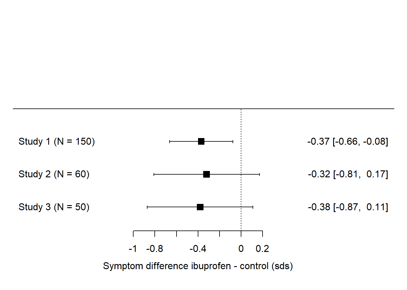
What we immediately see here is that all three studies produce about the same estimate - that ibuprofen produces lower depressive symptoms than control treatment by around 0.3 to 0.4 standard deviations. In study 1, this is enough to be significantly different from zero, because the sample size in study 1 is quite big, and hence the precision of parameter estimation is decent, so the confidence interval does not include zero. Studies 2 and 3 have smaller sample sizes, hence their precision is worse and the -0.3 to -0.4 is estimated with zero within its confidence interval. But, although the ‘significance’ is different between study 1 and studies 2 and 3, the actual findings are very similar. In fact, the ‘non-significant’ finding of study 3 has a larger effect size than the ‘significant’ one in study 1!
Here is the problem with vote counting. If you counted significance you would say ‘the evidence is mixed, with more studies failing to find an effect than studies finding one’. On the other hand, if you look at the actual parameter estimates, then the evidence is not remotely mixed: all studies concur that the effect is in the range of -0.3 or -0.4 standard deviations. And, surely, three independent estimates all in this narrow range ought to give you high confidence that the true effect is around here. You ought to have more confidence that there is an effect when you have added the evidence of studies 2 and 3 than you did when you just had study 1. But if you do vote-counting based on significance, then the opposite happens: your initial belief on the basis of ‘significant’ study 1 is eroded by the ‘non-significant’ studies 2 and 3.
There are even cases where none of the studies finds a significant effect, but the combined evidence suggests there is one. Imagine in our ibuprofen example if the forest plot had looked like this instead:
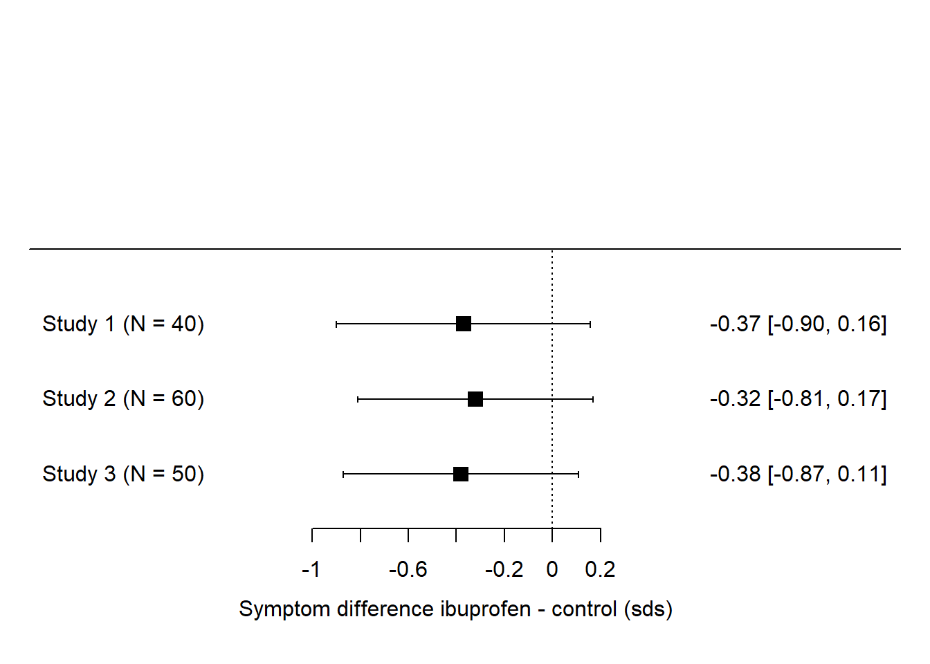
Here, none of the effects is ‘significant’ (i.e. not significantly different from zero) and so, in terms of vote counting, it’s a landslide for ‘no effect’. But, the studies are all pretty small. They all find parameter estimates in the -0.3 to -0.4 range, just with a broad confidence interval. We feel intuitively that the precision of the three studies considered together ought to be a lot better than any one of them considered individually. If we assume that our best estimate of the true effect size is somewhere close to the average of the estimates from the three studies, say around -0.34, and that the confidence interval for the three combined is smaller than for any one of the studies individually, then these three ‘non-significant’ studies actually seem to be telling us that there might be a significant effect.
Just as vote counting can make us believe there is no meaningful effect when there probably is one, it can make us believe there is a meaningful effect when there probably isn’t.
Let’s imagine a case where there are a couple of very small studies finding large effects, and then one much more serious follow up finding en effect close to zero. It could look like this:
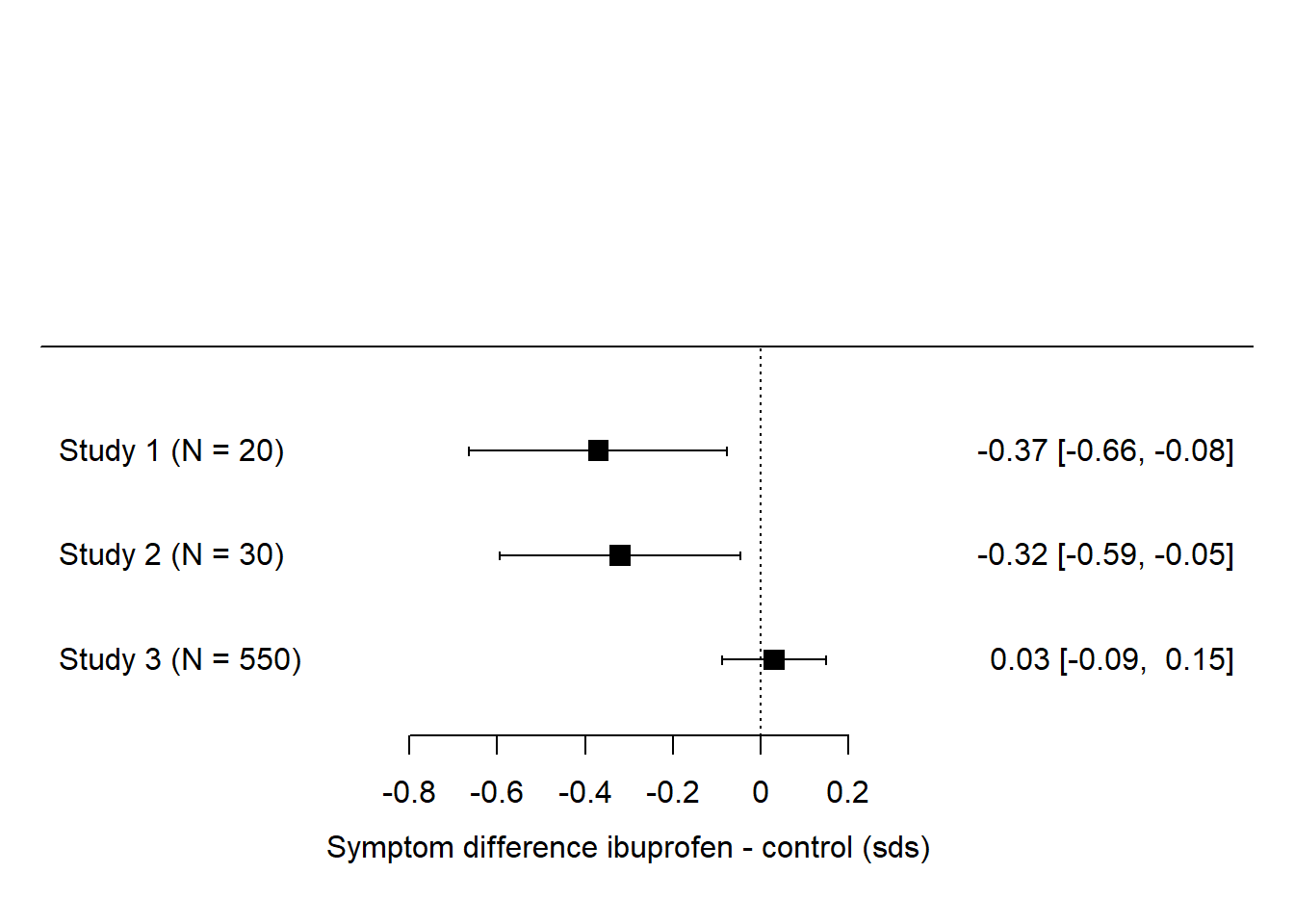
Here, two out of three had ‘significant’ effects, so vote-counting favours the hypothesis of an effect. But, if you consider the total number of people who have actually been studied, just 50 of them went into the studies claiming an effect, whereas 550 of them went into a study finding an effect size very close to zero. If the votes were weighted by the number of participants, and hence the amount of evidence, in the study, then study 3 would count a lot more than studies 1 and 2 combined.
17.3 Introducing metaanalysis
17.3.1 What metaanalysis is…..
The preceding section has shown you why vote-counting on the basis of significance is such a bad idea, and probably given you an inkling of how metaanalysis models work. In their simplest form, metaanalysis models combine estimates of the same parameter from multiple datasets in order to produce an overall effect size that integrates all the available evidence.
In particular, in the calculation of the overall effect size, estimates are weighted according to their precision, with more precise estimates (generally coming from studies with larger sample sizes) having greater influence than less precise estimates. The model also gives a confidence interval for the overall effect size, which is generally smaller than the confidence interval for the parameter estimate of any of the constituent studies.
Getting an overall effect size is the most basic thing you can do with a metaanalysis. You can also use the model to investigate heterogeneity in effect size (do the studies’ effect sizes differ from one another more than you would expect by chance given their sample sizes?); and also to ask whether any characteristics of the individual studies - their methodology or measurement for example - predict what size of effect they find. This is known as metaregression. Here, we are just going to cover the very basics.
17.3.2 And what you need to do it…..
In order to carry out a metaanalysis, all you need is the following two things:
A vector of effect sizes, one from each of your datasets or studies. The effect sizes can be in a number of formats: parameter estimates (either standardized or not); differences in means (usually standardized); correlation coefficients; or odds ratios. They capture the magnitude of effect or association for the phenomenon of interest from each study. Obviously, they all have to represent measurements on the scale. You cannot compare an effect size in terms of numbers of centimetres growth to another effect size in terms of millimetres of growth. They also all need to be estimates of the same type. If however the different analyses you are drawing from produced different types of estimate (for example, a standardized difference in means in one case and a odds ratio in the other), don’t despair. There are formulas available for the conversion of many types of effect sizes into a common currency like the correlation coefficient. The contributed R package
effectsizewill make many of these conversions for you.A vector of precisions, one for each of your effect sizes. The easiest way of capturing precision is the standard error of your parameter estimate, which you can find in your output from
lm(),lmer()andglm()objects in R (or, its square, which is known as the sampling variance). An alternative way of representing the precision is to know the lower bound and upper bound of the 95% confidence interval for each of your parameter estimates. You can convert between these two formats by remembering that the difference between a parameter estimate and either bound of its confidence intervals is generally 1.96 times its standard error. (Though, be careful when applying this rule of thumb for odds ratios; there it applies on the log odds scale, but ceases to supply when you convert from log odds to odds, as people often do when reporting their results). For continuous variables, if you don’t have a standard error, but do have the number of people in each group plus the standard deviation of the measurement, you can easily get the standard error you need.
Armed with these two pieces of information, it is very easy to run a metaanalysis, as we will see in the following examples. There are a number of contributed R packages, but I recommend the one called metafor.
There are two cases where you might use meta-analysis: where you are drawing the different estimates from the literature; and where you are wanting to integrate the information from several of your own studies. We will work through an example of each.
17.4 Metaanalysis case 1: studies from the literature
In this example, we are going to imagine we are doing a metaanalysis of studies on whether taking part in mindfulness meditation increases the physiological activity of an enzyme called telomerase. Telomerase is involved in cellular repair; you can think of it informally as reversing the effects of ageing and damage. Thus, to cut a complex story short, increasing its activity should generally be associated with better health and slower ageing in the long run. Meditation has been observed to be correlated with better health; these studies are driving to delve into the mechanisms by which such an effect, if it is causal, could come about.
For the sake of the example, we are going to assume we have done a systematic search and found three studies (Lavretsky et al. 2013; Daubenmier et al. 2012; Ho et al. 2012). In reality there are more than three, but these three are sufficient for an illustration. We return to how you would have got to your set of three at the end of the section.
17.4.1 Working out what data to extract
Having established your set of studies (in this case, three), the first thing to do is to read them all and ask yourself the question: is there some statistic they all report that is comparable? Only if you can find such a common currency can you complete your metaanalysis. It’s usually a bit messy since the reporting of different studies is so variable, you have to make some judgements, and sometimes you have to compare the only-roughly-comparable, as you will see here. Sometimes you have one type of effect size estimate (say a correlation coefficient) from some of your studies, and a different type (say an odds ratio) from others. In such a case you will have to use conversion formulas, such as those available through the effectsize package.
Here, all three studies include a control group who did not do mindfulness meditation and a treatment group who did. They all measured telomerase activity before and after the treatment in both groups. Then they do various statistical tests, not necessarily the same one. However, all report, in their tables, some descriptive statistics of telomerase activity values in each group after the treatment, and we can make use of these. Let’s have a look at the relevant parts of the papers.
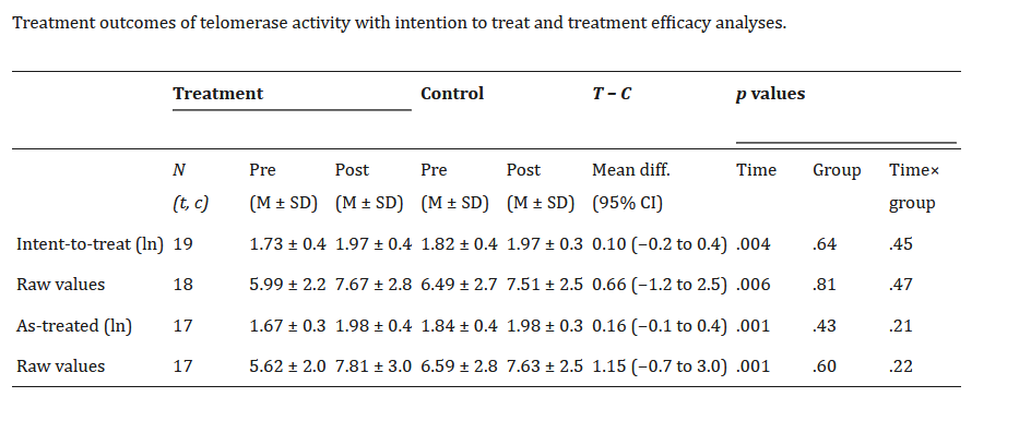

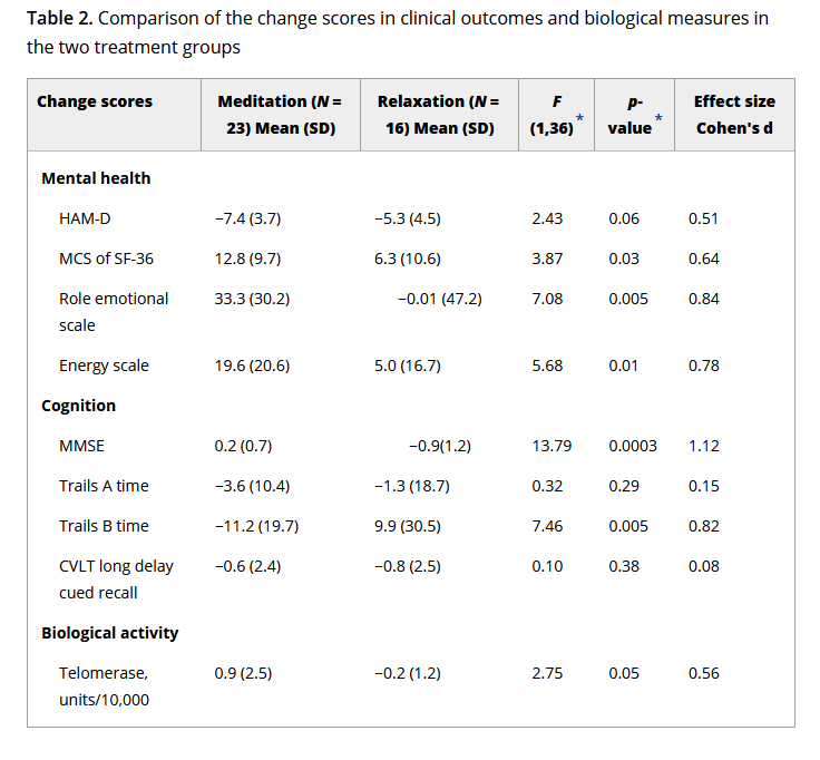
The first study gives you a choice of raw telomerase values, or log-transformed ones. Since the other studies don’t give the log-transformed ones, we will have to prefer the raw ones. It also defines the groups in two different ways: intention to treat (group membership as originally assigned); and as treated (what the participants actually did). These are not identical since someone was assigned to do the meditation but did not actually do it. We will go with intention to treat; it is not going to make much difference, and it is conservative in terms of estimating the effect size.
The second study gives us mean and standard deviation of telomerase activity for the two groups after the intervention. We can make this comparable with the first study.
The third study gives us the mean and standard deviation of telomerase change over the course of the trial for each group. That is, they have substracted each individual’s telomerase at baseline from their telomerase after the trial, and reported this difference. The mean and standard deviation of change score by group are related but not identical to the mean and standard of post-trial telomerase by group. The differences between the two group means are, in expectation, the same in the two cases. Since assignment is random, the expected value of the difference between the groups is zero at baseline, whereas after the intervention, the expectations of the two means differ by the expected value of change associated with the treatment. However, the standard deviation of change in telomerase within an individual over a few months is not really the same quantity as the standard deviation of telomerase across individuals.
Nonetheless, we are going to have to work with this. We are going to have to compare the group difference in post-trial telomerase for studies 1 and 2 with the group difference in telomerase change score for study 3. In my experience of metaanalysis, you have to make a constant series of small decisions like this in order to get anywhere at all, and often you are not exactly comparing like with like. Of course, it is much better if all studies openly archive their data in a repository. Then, you can go to the raw data and extract the exact same statistics from each one, in order to make your set of effect sizes more exactly comparable.
17.4.2 Extracting the data
So, we have some kind of mean and standard deviation of telomerase activity per group after the trial, and we have standard deviations of this within each group (of level, for studies 1 and 2; of change for study 3). This means that we can calculate a standardized mean difference (SMD) statistic, and its corresponding precision, for each study. The SMD is the difference between the groups expressed in units of the pooled standard deviation observed in the study. So, for example, an SMD of 1 means that the treatment group had telomerase activity 1 deviation higher than the control group after the trial; zero means no difference; -0.5 means their activity was half a standard deviation lower, and so on. We express the difference in terms of standard deviations rather than in terms of actual units of telomerase activity per microlitre of blood, because the absolute numbers could be very different from study to study, for example if the lab equipment worked in different ways, the samples were prepared differently, and so on. By always comparing in terms of standard deviations observed within that study, you abstract away from these measurement differences.
To obtain the SMD, we need the means and standard deviations for each group, and also the number of participants in each group. Though these ns are not shown in the tables, they can be found in the three papers. Often, it’s quite hard to get the exact numbers, since some participants have missing data for some variables or time points, and the reporting is never quite as explicit as it could be. This is another reason for providing your raw data.
Once we have identified the information we need, we start to make a data frame of the information from our three studies; something like this:
telo.data <- data.frame(
  studies = c("Daubenmier et al. 2012", "Ho et al. 2012", "Lavretsky et al. 2012"),
  mean.treatment = c(7.67, 0.178, 0.90),
  mean.control = c(7.51, 0.104, -0.2),
  sd.treatment = c(2.8, 0.201, 2.5),
  sd.control = c(2.5, 0.069, 1.2),
  n.treatment = c(19, 27, 23),
  n.control = c(18, 25, 16)
    )
Lets see our data:
##                  studies mean.treatment mean.control
## 1 Daubenmier et al. 2012          7.670        7.510
## 2         Ho et al. 2012          0.178        0.104
## 3  Lavretsky et al. 2012          0.900       -0.200
##   sd.treatment sd.control n.treatment n.control
## 1        2.800      2.500          19        18
## 2        0.201      0.069          27        25
## 3        2.500      1.200          23        16
17.4.3 Calculating your effect sizes
To calculate our SMDs, we need the contributed package we are going to use for our metaanalysis, metafor.
## Error in install.packages : Updating loaded packagesThe metafor package has a function called escalc() which spits out effect sizes in various formats. We specify that measure="SMD" in calling escalc() to indicate that it is the SMD we want. (Two closely related versions of the SMD are Cohen’s d and Hedges’ g; the escalc() function spits out Hedges’ g.) We have to tell the escalc()function to find the mean for each group, the sds for each group, and the ns for each group. Which group you select for group 1 here will determine whether your effect sizes will come out positive (i.e. a positive number when the treatment group is higher than the control) or negative (i.e. a positive number when the control group is higher than the treatment group).
telo.effect.sizes = escalc(measure ="SMD",
       m1i = telo.data$mean.treatment,
       m2i = telo.data$mean.control,
       sd1i = telo.data$sd.treatment,
       sd2i = telo.data$sd.control,
       n1i = telo.data$n.treatment,
       n2i = telo.data$n.control)
In your object telo.effect.sizes you should have the three SMD values, 0.0589. 0.4775, 0.5196, and their three sampling variances, 0.1082, 0.0792, 0.1094. The sampling variance is the square of the standard error. It would be neater to put these into the original data frame telo.data, so let’s do this.
##                  studies mean.treatment mean.control
## 1 Daubenmier et al. 2012          7.670        7.510
## 2         Ho et al. 2012          0.178        0.104
## 3  Lavretsky et al. 2012          0.900       -0.200
##   sd.treatment sd.control n.treatment n.control
## 1        2.800      2.500          19        18
## 2        0.201      0.069          27        25
## 3        2.500      1.200          23        16
##           yi         vi
## 1 0.05888342 0.10823399
## 2 0.47753912 0.07922976
## 3 0.51962890 0.10943998
17.4.4 Running the metaanalysis
Now it is time to fit the metanalysis model, which we do with the function rma() from metafor. We specify where we want it to look for the effect size values yi and the sampling variances vi.
##
## Random-Effects Model (k = 3; tau^2 estimator: REML)
##
##   logLik  deviance       AIC       BIC      AICc
##  -0.1420    0.2839    4.2839    1.6702   16.2839
##
## tau^2 (estimated amount of total heterogeneity): 0 (SE = 0.0975)
## tau (square root of estimated tau^2 value):      0
## I^2 (total heterogeneity / total variability):   0.00%
## H^2 (total variability / sampling variability):  1.00
##
## Test for Heterogeneity:
## Q(df = 2) = 1.2441, p-val = 0.5368
##
## Model Results:
##
## estimate      se    zval    pval   ci.lb   ci.ub
##   0.3652  0.1796  2.0331  0.0420  0.0131  0.7172  *
##
## ---
## Signif. codes:  0 '***' 0.001 '**' 0.01 '*' 0.05 '.' 0.1 ' ' 1
In the interest of transparency, you should get identical results by giving rma() the standard errors rather than the sampling variances:
##
## Random-Effects Model (k = 3; tau^2 estimator: REML)
##
##   logLik  deviance       AIC       BIC      AICc
##  -0.1420    0.2839    4.2839    1.6702   16.2839
##
## tau^2 (estimated amount of total heterogeneity): 0 (SE = 0.0975)
## tau (square root of estimated tau^2 value):      0
## I^2 (total heterogeneity / total variability):   0.00%
## H^2 (total variability / sampling variability):  1.00
##
## Test for Heterogeneity:
## Q(df = 2) = 1.2441, p-val = 0.5368
##
## Model Results:
##
## estimate      se    zval    pval   ci.lb   ci.ub
##   0.3652  0.1796  2.0331  0.0420  0.0131  0.7172  *
##
## ---
## Signif. codes:  0 '***' 0.001 '**' 0.01 '*' 0.05 '.' 0.1 ' ' 1
So what does the model show? The estimate of 0.3652 means that our synthetic estimate, taking all three data sets into account, is that meditation has an effect of telomerase activity with a standardized mean difference of about 0.37, and a 95% confidence interval of 0.01 to 0.72. Notice that this confidence interval does not include zero, and so we say that the combined evidence is for a significant effect of meditation.
What else does the model tell us? The heterogeneity test (Q) is not significant and the heterogeneity statistic I^2 is estimated at 0%. These statistics mean, in effect, that the results of the studies do not differ any more from one another than would be expected given that they are extremely small, and small studies find variable results even when the underlying effect is constant. These statistics become more interesting in much larger metaanalyses, where studies may find quite different results depending on their methods or the populations they are done in.
Now, let’s get the forest plot:
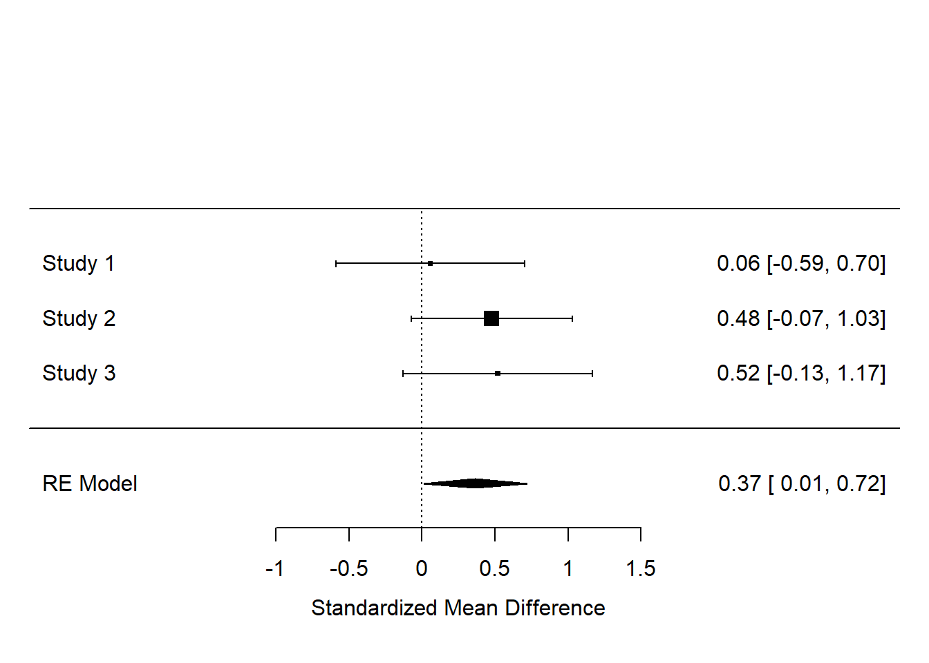
We can make it a bit nicer by telling the forest() function where to look for the names of the studies:
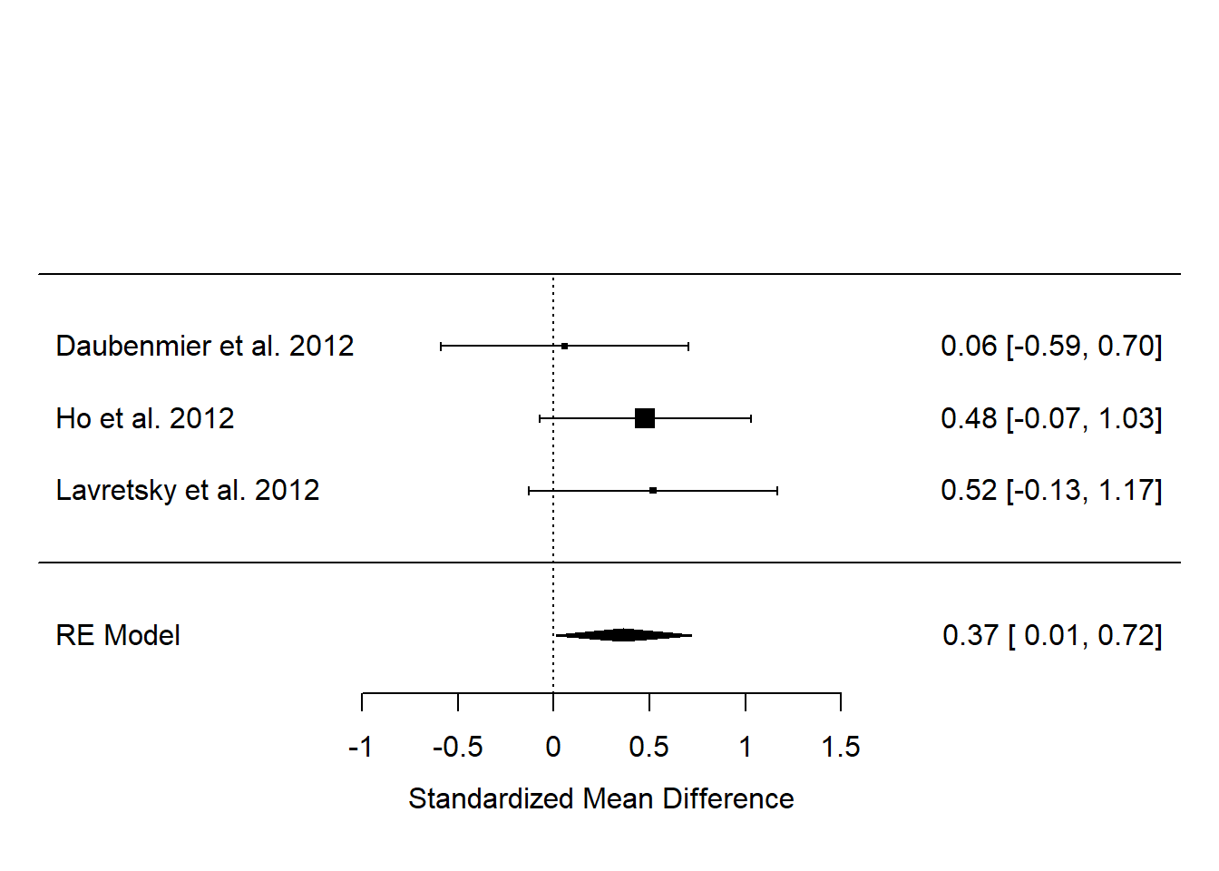
So, although, by our analysis, none of the three studies has an effect estimate significantly different from zero, the results overall suggest there is an effect, whose best estimate is 0.37, with a 95% confidence interval from 0.01 to 0.72.
Something you might have noticed is that the claims about significance for the individual studies implied in the forest plot seem to be at odds with what the papers said. For example, Daubenmeir et al. reported no significant effect (and we concur), but both Ho et al. and Lavretsky et al. claimed their effects as significant, whereas we show their 95% confidence intervals as crossing zero. In both cases, this is because they performed more sophisticated analyses than our simple SMD, adjusting for more things, that make their precisions better. But, we had to use SMD since although it is basic we could get some version of it for every study. The point of metaanalysis is that the significance of individual studies is not terribly important; it’s the overall estimate that you are interested in, and in this, the overall evidence suggests that the claims Ho et al. and Lavretsky et al. made from their individual studies were probably generalizable.
17.4.5 Reporting the metaanalysis
I would report the results in something like the following way. ’We combined the standardized mean difference estimates from the three studies and performed a random effects metaanalysis. The estimated overall effect size was 0.37 (95% confidence interval 0.01 to 0.72), suggesting evidence that meditation increases telomerase activity relative to control. There was no evidence for heterogeneity across studies (\(Q^2(2)\) = 1.24, p = 0.54; \(I^2\) = 0%).
I would then show the forest plot.
17.4.6 Systematic reviewing
For this example, I just assumed that you had come to the conclusion that there were these three studies and no others to be included in your metaanalysis. How would you get to this point in reality?
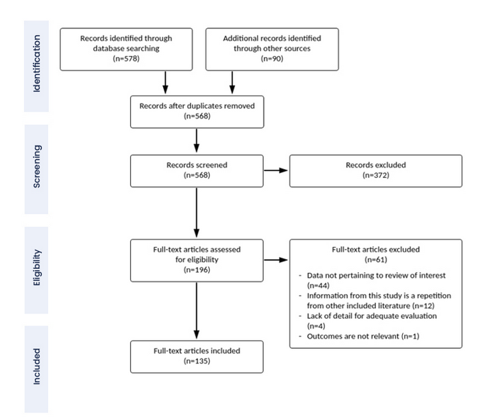
You would do so by systematic reviewing. In systematic reviewing, you perform a verifiable and replicable set of procedures to arrive at your set of candidate studies. Typically, this involves defining a set of search terms; using them to search online databases of scientific studies; screening the hits you found to determine which of these really meet the criteria needed to provide evidence on your question; then extracting the information from each one. Systematic reviewing is a whole discipline in its own right and I will not cover it in detail here. It often involves a lot of agonising about what a study really has to contain to constitute evidence on your exact question rather than a related one.
The point, though, is that it is not sufficient to merely assert that there are three studies providing evidence on the question. Instead, you have to show that you made some kind of objective, thorough and repeatable attempt to find all the evidence, and documented how you did that. Someone else should be able to repeat your systematic review and find the same sources.
An important part of a systematic review and metaanalysis is the PRISMA diagram. This identifies the steps in the reviewers’ workflow, showing exactly how the final the set of included studies was identified. I include one below (not related to the present example), just to show you what one looks like.
The combination of systematic reviewing and metaanalysis as an approach to understanding what we know has been an important improvement in knowledge-gathering in the last few decades, particularly in the medical sciences where it came from. Metaanalysis and systematic reviewing are part of a set of tools that offers to make our science more reliable and more cumulative. These days a medical or epidemiological finding is not credible until there are many studies and metaanalyses.
This is how it should be, though it is not without its problems. There are many small judgement calls to be made in the process of doing a metaanalysis, and a lot of researcher degrees of freedom. This means that different teams of metaanalysts can and sometimes do approach the same body of knowledge and come to rather different conclusions; or that the whole field becomes convinced of something because of a metaanalysis whose results depended on very specific (and non-obvious) researcher decisions. In many areas there are now metaanalyses of metaanalyses! In any event, if you do metaanalysis seriously you should pay great attention to replicability, and robustness or results to analytical and methodological decisions.
Still, as a method of evidence synthesis, systematic reviewing and metaanalysis knock narrative reviewing into a cocked hat.
17.5 Meta-analysis case 2: Mini-metanalysis of you own experiments
The other situation where metaanalysis can be very useful is within your own series of studies. You will often study the same effect or association in multiple datasets as you proceed, perhaps introducing additional refinements or recruiting multiple sets of participants. In this case, as in the case of reviewing the literature, it is less important to count whether the results were significant or not each time, and more important to synthesize the effect sizes from all the studies to get an overall metaanalytic estimate of the effect. This is called mini-metaanalysis or internal metaanalysis (Goh, Hall, and Rosenthal 2016).
You perform mini-metaanalysis in exactly the same way as metaanalysis from the literature, except that you have the advantage of having all the raw data at your finger tips, and hence being in a better position to extract optimal and comparable estimates from each data set.
I am going to show you this now with a very quick example from a paper we have already met (Nettle and Saxe 2020). As you may recall, in this paper, the authors were studying the effect of various features of a society on people’s intuitions about the extent to which resources within that society should be redistributed (i.e. shared out equally). One of those features was the society’s cultural heterogeneity, which was manipulated in the first five of the seven studies. Those studies differed in other ways, but they all had a manipulated heterogeneity vs. homogeneity variable, and they all measured basically the same outcome. Thus, we can synthesize the effects of this variable across all five.
The five experiments all featured within-subjects manipulation of heterogeneity vs. homogeneity, and a continuous outcome (ideal redistribution on a scale of 1-100). For a comparable effect size across the five, therefore, I am going to use the parameter estimate (and its standard error) for the heterogeneity IV, from a Linear Mixed Model, using a random effect for participant. I will include the other IVs from each study in the models, though they are not of interest in the mini-metanalysis.
17.5.1 Preparing the mini-metaanalysis
First, I go to the paper’s OSF repository (https://osf.io/xrqae/) and save the data files for the first five studies (study1.data.csv,…study5.data.csv) to my local working directory.
Now let’s load in the data.
## New names:
## Rows: 600 Columns: 18
## ── Column specification
## ────────────────────────────────── Delimiter: "," chr
## (4): participant, luck, heterogeneity, gender dbl (12):
## ...1, level, mode, age, left.right, support.... lgl (2):
## passed.luck.comprehension, passed.het.compre...
## ℹ Use `spec()` to retrieve the full column specification
## for this data. ℹ Specify the column types or set
## `show_col_types = FALSE` to quiet this message.
## • `` -> `...1`## New names:
## Rows: 800 Columns: 19
## ── Column specification
## ────────────────────────────────── Delimiter: "," chr
## (5): participant, luck, heterogeneity, viewpoint,... dbl
## (12): ...1, level, mode, age, left.right, support.... lgl
## (2): passed.luck.comprehension, passed.het.compre...
## ℹ Use `spec()` to retrieve the full column specification
## for this data. ℹ Specify the column types or set
## `show_col_types = FALSE` to quiet this message.
## • `` -> `...1`## New names:
## Rows: 800 Columns: 20
## ── Column specification
## ────────────────────────────────── Delimiter: "," chr
## (5): participant, luck, heterogeneity, war, gender dbl
## (12): ...1, level, mode, age, left.right, support.... lgl
## (3): passed.luck.comprehension, passed.het.compre...
## ℹ Use `spec()` to retrieve the full column specification
## for this data. ℹ Specify the column types or set
## `show_col_types = FALSE` to quiet this message.
## • `` -> `...1`## New names:
## Rows: 400 Columns: 22
## ── Column specification
## ────────────────────────────────── Delimiter: "," chr
## (3): heterogeneity, war, gender dbl (19): ...1,
## participant, level, age, left.right, s...
## ℹ Use `spec()` to retrieve the full column specification
## for this data. ℹ Specify the column types or set
## `show_col_types = FALSE` to quiet this message.
## • `` -> `...1`Now, let’s make sure that in each data set, we have the heterogeneity variable set up so that the reference category is Homogeneous, and therefore that the parameter estimate will reflect the departure from the reference level when the variable is at the level Heterogeneous.
d1$heterogeneity <- factor(d1$heterogeneity, levels=c("Homogeneous", "Heterogeneous"))
d2$heterogeneity <- factor(d2$heterogeneity, levels=c("Homogeneous", "Heterogeneous"))
d3$heterogeneity <- factor(d3$heterogeneity, levels=c("Homogeneous", "Heterogeneous"))
d4$heterogeneity <- factor(d4$heterogeneity, levels=c("Homogeneous", "Heterogeneous"))
d5$heterogeneity <- factor(d5$heterogeneity, levels=c("Homogeneous", "Heterogeneous"))
Now, let’s fit our mixed models, one for each study. We have additional predictors as well as heterogeneity from each study, depending on that study’s particular design, but let’s always put our predictor of interest first in each model. Note also that I am going to scale the outcome variable, so the parameter estimates are in terms of standard deviations of the outcome.
library(lmerTest)

m1 <- lmer(scale(level)~ heterogeneity + luck + (1|participant), data=d1)
m2 <- lmer(scale(level)~ heterogeneity + luck + (1|participant), data=d2)
m3 <- lmer(scale(level)~ heterogeneity + luck + viewpoint + (1|participant), data=d3)
m4 <- lmer(scale(level)~ heterogeneity + luck + war + (1|participant), data=d4)
m5 <- lmer(scale(level)~ heterogeneity + war + (1|participant), data=d5)
Look at the summary for m1.
## Linear mixed model fit by REML. t-tests use
##   Satterthwaite's method [lmerModLmerTest]
## Formula:
## scale(level) ~ heterogeneity + luck + (1 | participant)
##    Data: d1
##
## REML criterion at convergence: 1604.9
##
## Scaled residuals:
##      Min       1Q   Median       3Q      Max
## -2.42719 -0.62971  0.00556  0.63994  2.58273
##
## Random effects:
##  Groups      Name        Variance Std.Dev.
##  participant (Intercept) 0.2380   0.4879
##  Residual                0.6936   0.8328
## Number of obs: 600, groups:  participant, 100
##
## Fixed effects:
##                             Estimate Std. Error        df
## (Intercept)                  0.42684    0.08369 325.95403
## heterogeneityHeterogeneous  -0.13818    0.06800 497.00000
## luckLow                     -0.62332    0.08328 497.00000
## luckMedium                  -0.44994    0.08328 497.00000
##                            t value Pr(>|t|)
## (Intercept)                  5.100 5.76e-07 ***
## heterogeneityHeterogeneous  -2.032   0.0427 *
## luckLow                     -7.485 3.29e-13 ***
## luckMedium                  -5.403 1.02e-07 ***
## ---
## Signif. codes:
## 0 '***' 0.001 '**' 0.01 '*' 0.05 '.' 0.1 ' ' 1
##
## Correlation of Fixed Effects:
##             (Intr) htrgnH luckLw
## htrgntyHtrg -0.406
## luckLow     -0.498  0.000
## luckMedium  -0.498  0.000  0.500
The numbers you are going to want are the -0.13818 (the estimate) and the 0.06800 (its standard error). You could just type these into a new data frame, but that would be silly, since we can pick them directly out of the model summary as follows:
## [1] -0.1381814And:
## [1] 0.06799793So, to make our data frame for the metaanalysis, we pick out the relevant numbers from all the models as follows:
redist.data <- data.frame(
  b = c(summary(m1)$coefficients["heterogeneityHeterogeneous", "Estimate"],
        summary(m2)$coefficients["heterogeneityHeterogeneous", "Estimate"],
        summary(m3)$coefficients["heterogeneityHeterogeneous", "Estimate"],
        summary(m4)$coefficients["heterogeneityHeterogeneous", "Estimate"],
        summary(m5)$coefficients["heterogeneityHeterogeneous", "Estimate"]),
  se = c(summary(m1)$coefficients["heterogeneityHeterogeneous", "Std. Error"],
        summary(m2)$coefficients["heterogeneityHeterogeneous", "Std. Error"],
        summary(m3)$coefficients["heterogeneityHeterogeneous", "Std. Error"],
        summary(m4)$coefficients["heterogeneityHeterogeneous", "Std. Error"],
        summary(m5)$coefficients["heterogeneityHeterogeneous", "Std. Error"])
  )
Have a look at this data frame and make sure you have the right things. If necessary, get the summaries of the individual models to see how the numbers relate.
##             b         se
## 1 -0.13818139 0.06799793
## 2 -0.08319039 0.06212917
## 3 -0.14319765 0.05220204
## 4 -0.16525021 0.05883491
## 5 -0.25103649 0.06446888
17.5.2 Running the mini-metaanalysis
Now it is a simple question of fitting your metaanalysis model.
##
## Random-Effects Model (k = 5; tau^2 estimator: REML)
##
##   logLik  deviance       AIC       BIC      AICc
##   5.6624  -11.3247   -7.3247   -8.5521    4.6753
##
## tau^2 (estimated amount of total heterogeneity): 0 (SE = 0.0026)
## tau (square root of estimated tau^2 value):      0
## I^2 (total heterogeneity / total variability):   0.00%
## H^2 (total variability / sampling variability):  1.00
##
## Test for Heterogeneity:
## Q(df = 4) = 3.6974, p-val = 0.4485
##
## Model Results:
##
## estimate      se     zval    pval    ci.lb    ci.ub
##  -0.1546  0.0270  -5.7272  <.0001  -0.2076  -0.1017  ***
##
## ---
## Signif. codes:  0 '***' 0.001 '**' 0.01 '*' 0.05 '.' 0.1 ' ' 1
So, overall, we find that manipulating the apparent cultural heterogeneity of the society reduces preferred redistribution by 0.1546 standard deviations, with a 95% confidence interval -0.2076 to -0.1017. There is no apparent heterogeneity across the studies beyond what would be expected by sampling variability, as indicated by the non-significant Q statistic, and the \(I^2\) estimate of 0.
We can also look at the results on a forest plot.
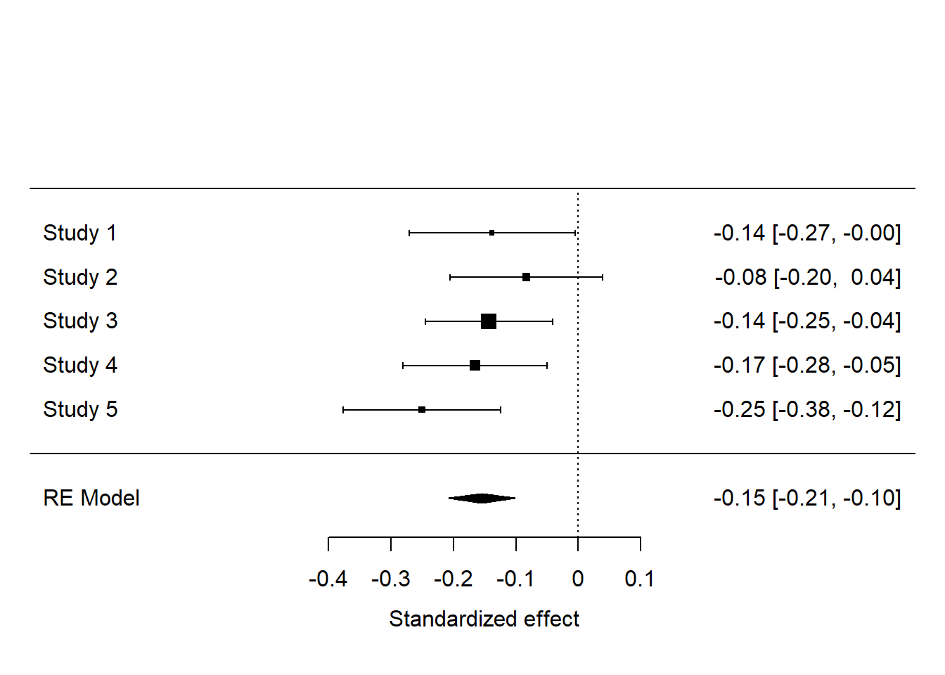
These results are super clear. Although there is some variation in significance in individual studies (the effect in study 2 was not significant), the studies amount to strong support for the existence of a small negative effect of manipulated heterogeneity on preferred redistribution.
17.5.3 What to do with mini-metaanalysis
Mini-metanalysis will be useful in many of your papers. These days it is good practice to have a replication study or two within your paper. And, you may go on to run variants and refinements within a series of studies, within each of which the same basic comparison is made. You should provide a mini-metanalysis so the reader can see what the evidence adds up to. You can include this in a separate section after the reporting of each individual study’s results. Or, you could consider replacing separate results sections on each individual study with just a meta-analysis. Analysis of studies separately could go into Supplementary Materials and the main results figure could be something like the forest plot shown above. It really contains all the information the reader needs, in a way that is a lot more concise than five separate results texts and five separate figures.
A question you might be asking is the following: when should I do mini-metaanalysis, and when should I simply combine the datasets from all the separate studies into one big dataset, and analyse that directly? This is a good question. In the case we have just been through, there were some methodological variations: the studies differed in terms of which other IVs they included, and in a number of other small methodological ways. So here it makes more sense to keep them separate but combine their results through metaanalysis. On the other hand, if your methods across several studies were absolutely identical or very nearly so, then you can combine all the datasets and do a single analysis. In such cases, meta-analysis and combined analysis should give you broadly the same answer in terms of the overall effect size.
17.6 Metaregression
The examples in this chapter have been exclusively concerned with using metaanalysis to produce an integrated estimate of an effect size from several datasets. This is only a small part of the use of metaanalysis though. More often, you want to explain variation in the effect sizes, using as predictors methodological features of the studies. This is called metaregression. You need more than 5 effect sizes to do this meaningfully, which is why I have not gone into it here. But the general outline is simple: you add extra columns to your data frame of effect sizes, in which you record your candidate predictors of variation in effect size. You then add these variables to your call to the rma() function using the argument mods = ~ variable1 + variable 2....
17.7 Summary
In this chapter, we have met the basic idea of metaanalysis and understood why it is a good way of synthesizing evidence– a much better way than vote counting on the basis of significance! We worked through examples in which we extracted evidence for metaanalyis from the literature; and in which the metaanalysis was internal synthesis of a series of our own studies. We also touched on related activities such as systematic reviewing and metaregression.