18 Simulations, writing R functions, and statistical power
18.1 Introduction
This chapter has several purposes. One is to convey the basics of writing your own functions in R, a useful skill to have. The second is to show you, in a simple case, how you could simulate the data from an experiment before performing it, and why this would be useful. The third is to introduce the principles of statistical power, which leads on to a discussion of power analysis and how to choose and justify your sample size.
18.2 Basics of simulating datasets
Let’s imagine that we want to see what our data might look like, for an experiment with a simple two-group, between-subjects design, with one continuous DV. Suppose we are considering running 50 participants per group, and we want to know what it might look like if our IV increased the DV by 0.2 standard deviations. Let’s assume our DV will be scaled, so it will have a standard deviation of 1. We can thus represent the case we are interested in as the DV having a mean of 0 in the control condition, and a mean of +0.2 in the experimental condition, with a standard deviation of 1 in both cases.
We can generate random numbers drawn from a Normal distribution with a specified mean and standard deviation with the function rnorm(). The three arguments you need to give this function are n , the number of values required, mean, the mean of the distribution, and sd, the standard deviation of the distribution. So, rnorm(n=50, mean=0, sd=1) gives you 50 values drawn from \(N(0, 1)\).
So, the following code is going to produce the data frame we need. I have commented it so that you can see what each line is doing.
# First set up the variable identifying which condition each participant belongs to
# The rep() function repeats the given element the required number of times:
Condition <- c(rep("Control", times =50), rep("Experimental", times=50))

# Now make the variable with the values of the DV
Outcome <- c(rnorm(n=50, mean=0, sd=1), rnorm(n=50, mean=0.2, sd=1))

# Now bind the two variables together in a data frame
simulated.data <- data.frame(Condition, Outcome)
We have our first simulated data set!
Now we can do things like make plots of what we see. Note that this plot will look different every time you run the code (and yours will look different from mine), because we are sampling different data points from the underlying distribution each time.
library(tidyverse)
ggplot(simulated.data, aes(x=Condition, y=Outcome)) +
  geom_boxplot() +
  theme_classic()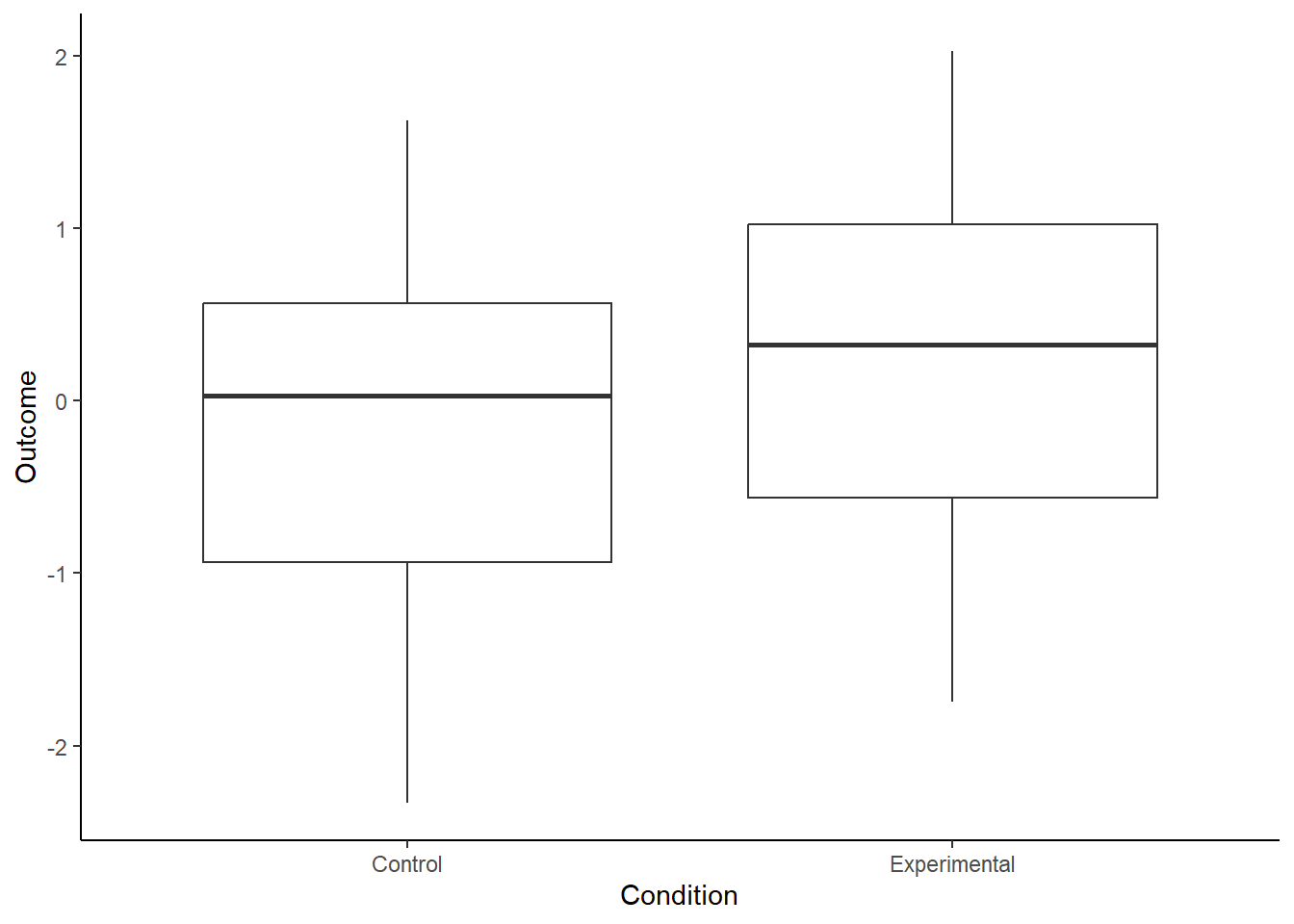
You may or may not see something going on, depending on the vagaries of sampling.
What about a statistical model? Here, you can try out the statistical model and test that you are planning for your real dataset when it comes.
##
## Call:
## lm(formula = Outcome ~ Condition, data = simulated.data)
##
## Residuals:
##     Min      1Q  Median      3Q     Max
## -3.3182 -0.6104  0.0880  0.6259  2.0256
##
## Coefficients:
##                       Estimate Std. Error t value
## (Intercept)            0.04886    0.14435   0.338
## ConditionExperimental  0.19229    0.20414   0.942
##                       Pr(>|t|)
## (Intercept)              0.736
## ConditionExperimental    0.349
##
## Residual standard error: 1.021 on 98 degrees of freedom
## Multiple R-squared:  0.008973,   Adjusted R-squared:  -0.00114
## F-statistic: 0.8873 on 1 and 98 DF,  p-value: 0.3485
Maybe you got a significant result, maybe not. Try re-running the chunk where you simulated the data, and then refitting model m1. Sometimes you will see it and sometimes (more often, actually) you will not. Most often your parameter estimate will be somewhere in the expected range, a small positive value, even if the test is not significant. With simulated data you are in a very unusual situation: you actually know the true value of the parameter that your model is estimating (i.e. 0.2). So you can get a really good sense of how far ‘off’ your understanding of the world can be in an experiment where you only have 50 participants per group.
18.3 Writing functions
Before we go any further with simulating data sets, I want to introduce you to writing your own functions. If you do complex simulations, your code will ends up hundreds of lines long and with lots of potential for error, unless you make it more economical by defining some functions to do in a single line the basic operations that you need to do repeatedly. Defining functions will allow you to code more economically, clearly, and with less risk of error.
18.3.1 The definition statement
To define your own function, you need a definition statement, in which you use a function called function() to set up the name, structure and arguments of your function.
Let’s make a simple function called simulate() that it going to make a new simulated data set in the way that in the first code chunk of this chapter. Having the function defined means that we can get a new dataset with a single line of code whenever we want (as long as during the session we have once run the definition statement. The {} encloses the body of the function (the steps that will actually be performed internally within the function every time it is called), and the return() statement specifies what the function “spits out” into the environment of your R session.
simulate <-function(n, effect.size) {
  Condition <- c(rep("Control", times =n), rep("Experimental", times= n))
  Outcome <- c(rnorm(n=n, mean=0, sd=1), rnorm(n=n, mean=effect.size, sd=1))
  return(data.frame(Condition, Outcome))
}
Now when we want a simulated data set, we just call simulate().
And, lo and behold, you have a new simulated data set called new.dataset in your environment to analyse.
18.3.2 Adding defaults
Our definition statement stipulates that any call of the simulate() function must provide the arguments n and effect.size. If you fail to provide either of these, you will get an error. Try the code below:
However, maybe there is a most frequent case you want to use your function to consider. Perhaps, you will usually want data sets with n=50 and effect.size=0.2 because this is what is most relevant to your experiment. In this case, you can set these values as default in the definition statement. This means that you won’t need to provide any values for those arguments when you call the function, in which case the defaults will be used; but you can do so if you wish, overriding the defaults.
You specify defaults by putting them in the definition statement as follows:
simulate <-function(n = 50, effect.size = 0.2) {
  Condition <- c(rep("Control", times =n), rep("Experimental", times= n))
  Outcome <- c(rnorm(n=n, mean=0, sd=1), rnorm(n=n, mean=effect.size, sd=1))
  return(data.frame(Condition, Outcome))
}
Now, if you want a data set with n = 50 and effect.size = 0.2, you don’t need to type these values, as they are supplied by default. In on the other hand you want any other value for these arguments, you can get it by saying so.
# Dataset1 will have an n of 50 and an effect size of 0.2
dataset1 <- simulate()
# Dataset2 will have an n of 100 and an effect size of 0.2
dataset2 <- simulate(n=100)
# Dataset3 will have an n of 50 and an effect size of 0.4
dataset3 <- simulate(effect.size=0.4)
# Dataset4 will have an n of 100 and an effect size of 0.4
dataset4 <- simulate(n=100, effect.size=0.4)
18.3.3 Returning to our simulation
Returning to our simulation, simulate data sets a few times and see what kind of results you get. For example you could run the code below repeatedly. Try to get a sense of how often you get a parameter estimate around 0.2, and how often you get a significant p-value. You can also play around with different values for n and effect.size.
##
## Call:
## lm(formula = Outcome ~ Condition, data = simulate())
##
## Residuals:
##      Min       1Q   Median       3Q      Max
## -2.20043 -0.67831 -0.04617  0.70378  1.95265
##
## Coefficients:
##                       Estimate Std. Error t value
## (Intercept)            0.06204    0.13924   0.446
## ConditionExperimental -0.02157    0.19691  -0.110
##                       Pr(>|t|)
## (Intercept)              0.657
## ConditionExperimental    0.913
##
## Residual standard error: 0.9846 on 98 degrees of freedom
## Multiple R-squared:  0.0001225,  Adjusted R-squared:  -0.01008
## F-statistic: 0.012 on 1 and 98 DF,  p-value: 0.913
Just running the simulation again and again is not very systematic, however. How about we run the simulation 100 times and ask (a) what parameter estimate do we get each time; and (b) is it significantly different from zero? How would we do this?
The code below will do the job. The comments explain how each line works.
# Set up two empty variables, Estimates that is going to contain the parameter estimates, and Significant which is going to say whether it was significant or not on each occasion
Estimate=NULL
Significant=NULL
# Define a for loop, R is going to loop through the material between the {} until index i reaches 100
for (i in 1:100){
  m <- lm(Outcome ~ Condition, data=simulate())
  # The next line line writes the parameter estimate from the current simulation to the variable Estimates
  Estimate[i] <- summary(m)$coefficients[2, 1]
  # The next line writes "Significant" to the variable Significant if p < 0.05, "Non-significant" otherwise
  # summary(m)$coefficients is the table that contains the p value, on the 2nd row at the 4th column
  Significant[i] <- ifelse(summary(m)$coefficients[2, 4]<0.05, "Significant", "Non-significant")
}
# The next line makes a data frame called Output with the results
Output <-data.frame(Estimate, Significant)
Ok, so now you should have a data frame called Output with 100 rows, each one giving you a parameter estimate from one simulated dataset, and whether it was significantly different from zero or not. Let’s get a sense of what happened. First, what did our parameter estimates look like:
##   mean(Estimate) sd(Estimate) min(Estimate) max(Estimate)
## 1      0.1908457    0.1954488    -0.2636834     0.6754664
Our mean parameter estimate is close to 0.2, which is reassuring, as 0.2 is the true value. But, we have a standard deviation of around 0.2 too, meaning that in a typical individual data set of 50 participants per group, our estimate of the parameter is off the true value by about 0.2 in either direction. And within the hundred data sets, we observe parameter estimates as discrepant as -0.26 and 0.68.
What about significance? How many times out of 100 did we observe a significant result?
##
## Non-significant     Significant
##              85              15
Not many! Only a bit better than what we would have expected if the true parameter had been zero (i.e. 5).
The other thing that we can do is to make a graph showing how our parameter estimate varies from simulation to simulation.
ggplot(Output, aes(x=Estimate, fill=Significant)) +
  geom_histogram(bins=10) +
  theme_classic() +
  ylab("Number of simulations") +
  #I am going to add a vertical line showing the true parameter value
  geom_vline(xintercept=0.2) +
  #And another dotted one at zero
geom_vline(xintercept=0, linetype="dotted") 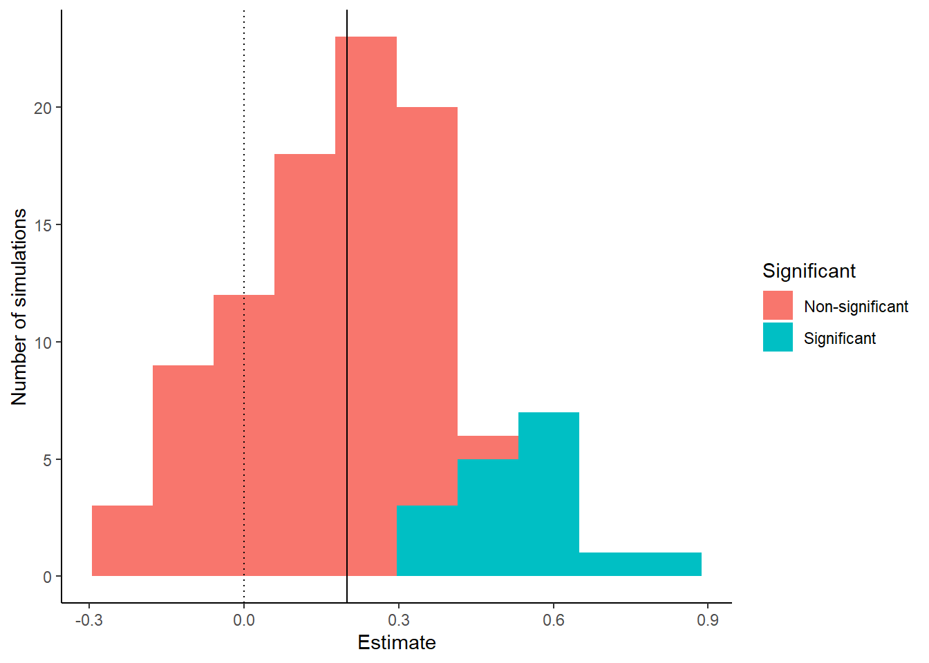
So, a few things should be clear. With 50 participants per group, in any individual data set we can be a long way off in our estimate of the effect of our manipulation. We can even be wrong about the direction of the effect. Plus, we rarely get a significant effect. In fact the only times we do get a significant are the times when, by chance, we had wildly overestimated the effect size. When our observed effect size is close to the true one, our test always returns “non-significant”! So, it should be immediately clear that 50 participants per group is not an adequate sample size for this experiment. We will return to this insight in the section on statistical power.
18.3.4 Making functions that call your functions
We are going to repeatedly need to run the code that generated the data frame Output, using different assumptions about n and effect.size. So, it would be useful to make a function that ran all that for us using one line. This means a function that calls our existing function simulate(). We make it using the code that follows. Note by the way that it is set up so that we give the values of n and effect.size to the outer function, hundred.sims() and they are in turn passed to the inner function simulate().
hundred.sims <- function(n = 50, effect.size = 0.2) {
Estimate=NULL
Significant=NULL
for (i in 1:100){
  m <- lm(Outcome ~ Condition, data=simulate(n = n, effect.size = effect.size))
  Estimate[i] <- summary(m)$coefficients[2, 1]
  Significant[i] <- ifelse(summary(m)$coefficients[2, 4]<0.05, "Significant", "Non-significant")
}
return(data.frame(Estimate, Significant))
}
Now, if we run hundred.sims() we are going to get the results from a hundred simulations with n=50 and effect.size=0.2. If we run hundred.sims(n=100), we are going to get the results from a hundred simulations with n=100 and effect.size=0.2. And so on: the hundred.sims() function allows you to vary n and effect.size as you wish.
18.4 Statistical power
Armed with our functions simulate() and hundred.sims(), it’s time to tackle the substantive topic of this chapter, statistical power. The statistical power of a test, given an effect size, is the probability that the test will detect that the effect is significantly different from zero if in fact the effect is there. So, our hundred.sims() function allows us to estimate statistical power for a given effect size and sample size in this experiment. The estimated power is simply the number of times out of the hundred that the result is significant.
We saw that with n=50 and effect.size=0.2, we usually don’t see a significant result. Let’s look at how the proportion of significant results changes as the true effect size gets bigger.
##
## Non-significant     Significant
## 86 14##
## Non-significant Significant
## 51 49##
## Non-significant Significant
## 19 81##
## Non-significant Significant
## 4 96What you should see is that as the effect size increases, the chance of detecting an effect significantly different from zero with n=50 gets bigger and bigger. You go from rarely doing so with effect.size=0.2 (power of around 20%) to almost always doing so with effect.size=0.8 (power of more than 95%). This gives us the first principle of statistical power: for a given sample size, the statistical power of a test increases with the size of the effect you are trying to detect.
How does varying our sample size impact our statistical power? I am sure you know that as your sample size gets bigger, your power to detect an effect of any given size gets better. Let’s try to visualize this. We will write a chunk of code that makes use of the hundred.sims() function that allows us to work out the estimated power to detect an effect size of 0.2, for a whole series of different sample sizes, and makes a graph. The chunk will put the data into an object called power.sample.size.data. The comments help you understand how the code is working. It may take a minute or two to run. After all, this code is performing thousands of simulations.
# We want to try all the sample sizes between 10 and 600 in jumps of 10
# The seq() function makes a sequence from the lower number to the high in intervals given by 'by'
Sample.Sizes <- seq(10, 600, by=10)
Power <- NULL
# Now make a loop that will step through the Sample Sizes
for (i in 1:length(Sample.Sizes)) {
  # Now d the current set of simulations for the sample size we are on
  Current.sim <- hundred.sims(n = Sample.Sizes[i], effect.size = 0.2)
  # Now figure out the power at the sample size we are on
  Current.power <- table(Current.sim$Significant)[2]
  # Now write this into the Power variable on the correct row
  Power[i] <- Current.power
  # Close the loop and moves on to the next sample size
}

# Record the data
power.sample.size.data <- data.frame(Sample.Sizes, Power)
Now, let’s make a plot of how power varies with sample size.
ggplot(power.sample.size.data, aes(x=Sample.Sizes, y=Power)) +
  geom_point() +
  geom_line() +
  theme_classic() +
  xlab("Sample size") +
ylab("Power estimated through simulation") 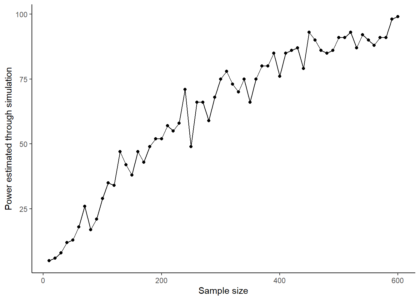
You can clearly see the second principle of statistical power in operation: power to detect an effect of a given size increases as the sample size increases. Here it goes from less than 20% at sample sizes of less than 50 per group, to almost but not quite 100% with sample sizes of 600 per group.
On our graph, there is some noise in the power-sample size relationship, which is due to the fact that you have only run 100 simulations at each sample size. If you wanted to smooth this, you could run 1000 simulations at each sample size. This would give you much more precise estimates and a smoother curve, but it would take ten times as long to run.
You can probably also discern that the power benefits of more participants gradually flatten out. The power gain of going from 50 to 150 looks bigger than the power gain of going from 450 to 550. This is because power generally increases with the square root of sample size. Your simulations confirm this. Let’s see this by replotting the graph, but with a square-root transformation of the x-axis, and a straight line of best fit through the data.
ggplot(power.sample.size.data, aes(x=Sample.Sizes, y=Power)) +
  geom_point() +
  geom_smooth(method="lm") +
  theme_classic() +
  xlab("Sample size") +
  ylab("Power estimated through simulation") +
  scale_x_sqrt()
## `geom_smooth()` using formula = 'y ~ x'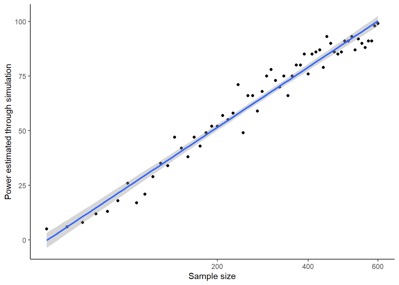
Why does power increase as sample size increases? It’s very simple: the precision of your parameter estimates gets better. You get estimates that have a smaller margin of error around the true value, and hence you can more often be confident that they differ from zero. Let’s visualize this by looking at the histogram of the parameter estimates from a hundred simulations with different sample sizes, coloured by whether they were significant or not. Again, the comments help you see what the code is doing.
# Run 100 simulations at each of four sample sizes
h50 <- hundred.sims(n=50)
h150 <- hundred.sims(n=150)
h250 <- hundred.sims(n=250)
h350 <- hundred.sims(n=450)
Estimates <- c(h50$Estimate, h150$Estimate, h250$Estimate, h350$Estimate)
Significance <- c(h50$Significant, h150$Significant, h250$Significant, h350$Significant)
# Make a variable indicating the sample size in each case
Sample.Sizes <- c(rep(50, times=100), rep(150, times=100), rep(250, times=100), rep(450, times=100))
# Put them in a data frame
Figure.data <- data.frame(Sample.Sizes, Estimates, Significance)
# Make the graph
ggplot(Figure.data, aes(x=Estimates, fill=Significance)) +
  geom_histogram(bins=10) +
  theme_classic() +
  ylab("Number of simulations") +
  geom_vline(xintercept=0.2) +
  geom_vline(xintercept=0, linetype="dotted") +
  facet_wrap(~Sample.Sizes)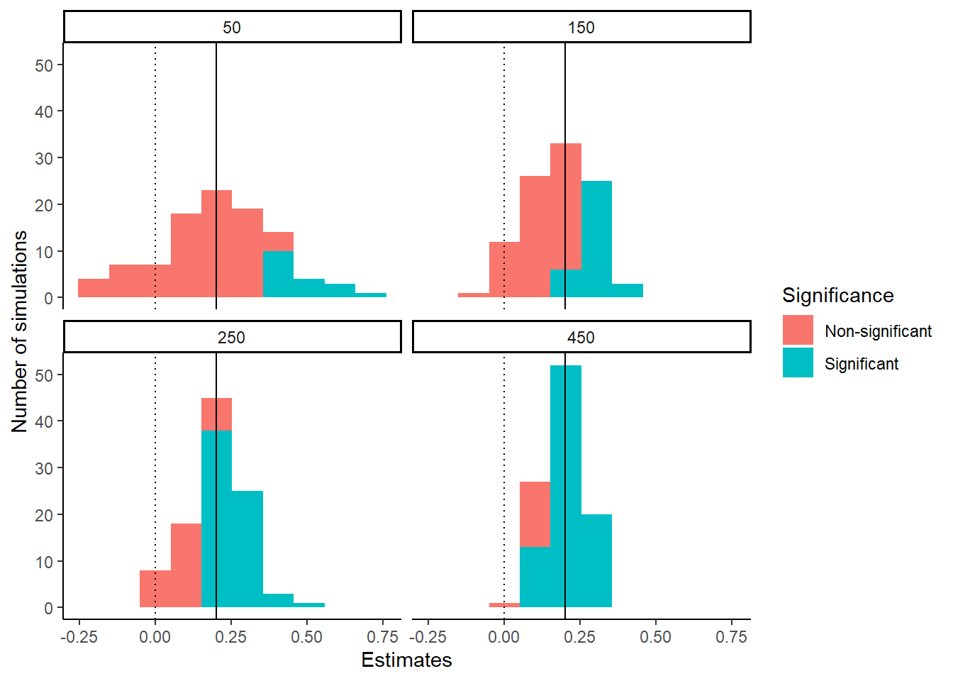
The reasons why larger sample sizes mean greater power are clear. In small samples, your parameter estimates vary widely from data set to data set. This is reflected in the large standard error of the parameter estimate, which means that your effects are rarely significant; in fact they are only significant where, by luck, you have massively overestimated the effect. As you move up in sample size, the variation in parameter estimate from data set to data set starts to be more modest; which means that more of them are significant since the standard error is smaller relative to the typical parameter estimate. By a sample size of 450, almost all of the estimates are significantly different from zero. More crucially, by a sample size of 450, all of the parameter estimates that are around the true value of 0.2 are classified as significantly different from zero. The experiment with 450 participants per group looks adequately powered to detect a sample size of 0.2 standard deviations. The experiment with 50 or 150 group definitely is not; though, you might be adequately powered to detect much larger effects at these smaller sample sizes. Power is defined only for the combination of an effect size and a sample size.
18.5 Using statistical power analysis
The previous section used simulation to introduce the main principles of statistical power. This section examines the ways you would use statistical power analysis in your work.
18.5.1 Analytical solutions for power
In the previous section, I used simulated datasets to estimate the power to detect effects of particular sizes at different sample sizes. In fact, it was not necessary for me to do this. For simple cases, there are mathematical formulas that give you the exact power of a test given the sample size and effect size. These formulas are available in the contributed package pwr, for example. So why did I approach power through simulation?
There are several reasons. It was a pretext for showing how to write your own R functions, which is a useful skill. Simulating datasets is useful for several reasons other than calculating statistical power. Doing so allows you to try out your analysis strategy and look at what your plots will look like under different assumptions about what you might find. Also, although power formulas exist for simple cases, they do not exist for complex scenarios that you might be trying to get a sense of: data sets with many variables, clustered structure, particular types of covariance between observations or variables. Being good at simulation can provide a tool for getting a sense of what such data sets might look like (or, the range of ways that they could look), and how to analyse them.
Finally, I find that approaching power through simulation is a really good way to understand it thoroughly.
Alright, now let’s say that we wanted to directly calculate power for the scenario considered in the previous section. Now is the time to run install.packages("pwr") if you have not done so before.
We use the pwr.t.test() function to calculate our power to detect an effect size of 0.2 standard deviations with a sample size of 50.
##
##      Two-sample t test power calculation
##
##               n = 50
##               d = 0.2
##       sig.level = 0.05
##           power = 0.1676755
##     alternative = two.sided
##
## NOTE: n is number in *each* group
It’s 0.17 or 17%. This should be pretty close to what you got by simulation.
In fact we can check the extent to which our simulations gave the same result as the formula. You should have the data frame power.sample.size.data in your environment. If not, regenerate it from the code chunk above.
We can add an extra column to that data frame, which is the power calculated exactly by pwr.t.test(). Note that we multiply by 100 because the output of pwr.t.test() is a proportion rather than a percentage.
power.sample.size.data$exact <- 100*pwr.t.test(n = power.sample.size.data$Sample.Sizes, d = 0.2)$powerNow let’s add the exact result to our graph as a red line.
ggplot(power.sample.size.data, aes(x=Sample.Sizes, y=Power)) +
  geom_point() +
  geom_line() +
  geom_line(aes(y=exact), colour="red") +
  theme_classic() +
  xlab("Sample size") +
ylab("Power estimated through simulation") 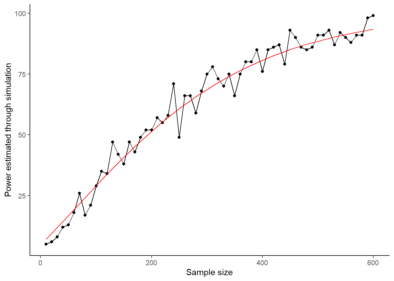
Our simulations did a pretty good job! But, for an immediate exact result in this simple case, you can go straight to pwr.t.test(). There are other formulas available in the pwr package, each of a different kind of situation and test. It’s worth getting acquainted with which one (if any) is suitable for your needs.
18.5.2 The main ways of using statistical power
Calculation of statistical power is used for the determination and justification of sample size. There are two main ways you might use it (see (Giner-Sorolla et al. 2024) for a more detailed discussion). The difference is whether you: start with an effect size that you want to be able to detect, and then work out what sample size you need to do so with adequate power; or start with a sample size that you have been or will be able to recruit, and then try to figure out what kind of effects you can detect with what power.
18.5.3 Sample size determination
Sample size determination analysis is the case where you don’t know your target sample size yet. You want to know what it ought to be. Having worked out your study design, you then need to specify a SESOI - a smallest effect size of interest. You put this into the power formulas, or a simulation, and ask: what size sample do I need to have a high chance of detecting the SESOI if it exists?
For example, let’s say you want to study the effects of ibuprofen on depressive symptoms. You could ask yourself: how much of an improvement would ibuprofen need to cause in order for it to be a useful part of medical treatment? Presumably if it improved symptoms by 0.01 standard deviations over three months (or something), this would not be very useful in treatment, even if technically not equal to zero. Perhaps we know that placebo pills, for example cause a symptom decrease of a certain magnitude. So the effect of ibuprofen might have to, say, 50% bigger than this before you would rate it as a useful discovery. You would set your SESOI appropriately.
Often you do not have a clear principle like clinical utility to guide you in setting the SESOI. If your study is a replication, you can look at the effect size observed in the study you are replicating. Sometimes there are still findings in the previous literature that help you benchmark the SESOI. For example, you might say ‘I know from previous literature that social isolation causes a 0.4 standard deviation increase in my outcome. I think my new manipulation of interest X is only important if causes an increase of at least this magnitude. If there is an effect, but it is smaller, then X is not important enough to pursue further. So I will power my study to be able to detect a SESOI of 0.4.’ .
If you really have nothing to go on, you could use the arbitrary values that are often employed: 0.2 standard deviations constitutes a small effect; 0.5 standard deviations a medium effect; and 0.8 standard deviations a large effect.
To give you a sense of what each of these means, consider the graphs below of how, in a simple experiment with two groups, the outcome values in the control and experimental conditions will overlap given small, medium and large effects.
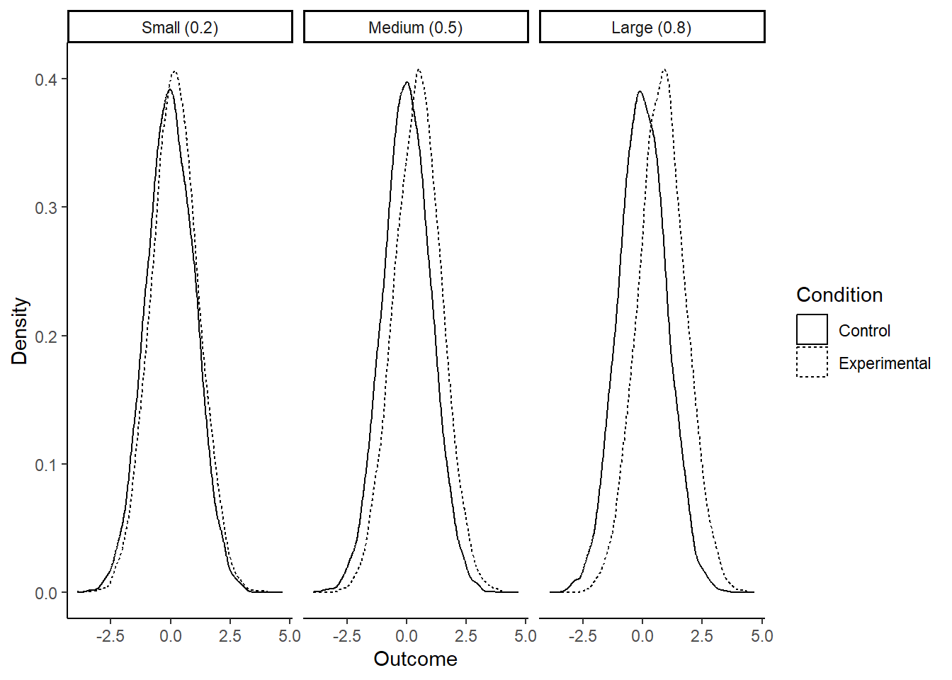
With a small effect (0.2), the means are slightly different, but frankly you need a microscope to see it. The distributions are still almost completely overlapping. Many values from the control condition are higher than many values from the experimental condition, and you certainly can say nothing about which condition a data point came from by looking at the outcome value.
With a large effect (0.8), the difference in means is much more obvious. If you guessed which condition a given data point came from based on its value, you would be right much more often than not. But still, even with an effect size of 0.8 standard deviations, the distributions are very overlapping. Your manipulation is certainly not a magic bullet, dwarfing other influences on the outcome.
In experimental studies (especially if you use between-subjects manipulation), if you power for a SESOI of 0.2 you will be running hundreds or even thousands of participants. You have to ask yourself if this is a good use of resources; if the effect is that small, is it really meaningful anyway? If you are testing a theoretical claim, I would be more tempted to reason as follows: my theory does not just say that X affects Y; it says that X is an important driver of Y. So if the theory is right, changing X ought to change Y by at least a medium effect size. Any less than this and the theory has failed. So, a fair test of the theory is to set my sample size to give me very good power to detect a medium effect size (0.5). If I then don’t see a significant effect, then either: X has no effect on Y, and the theory has failed; or X has only a very small effect on Y, and the theory has failed; or I’ve been really unlucky.
However, there are times when even a very small effect of X on Y, or association between X and Y, would be theoretically or practically interesting. In such a case, if you have the resources, you should set your sample size up to have good power to detect even a small effect size. But - I warn you - unless you have within-subjects manipulation, this can mean some very large samples.
One question I have glossed over. When I say ‘set your sample size to give you very good power to detect such-and-such an effect’, what does ‘very good power’ consist of? What is the power level I should insist on? It can’t be 100% because power only approaches 100% as the sample size tends to infinity; you never quite get there. If you set it at 95% (the obvious counterpart to the p = 0.05 criterion for significance), you end up spending a lot on running large samples, due to the marked flattening off of the sample size-power curve at its right-hand end. Many traditional statistics texts recommended 80%. Personally, I prefer 90%. If I am going to go to all the trouble of running a study, I would like to have more than an eight out of ten chance of seeing something interesting if it is actually there!
18.5.4 Power determination or minimal detectable effect calculation
The other major case of power analysis is where your sample size is set anyway, by your budget or time window or technology, or just by the number of individuals that are available in the population you are studying. Here, you can’t just decide on a SESOI and then determine the required sample size accordingly.
However, you can still use power analysis. You can say ‘given that my sample size is going to be n, then what level of power will I have to detect an effect of 0.5 standard deviations, or 0.2 standard deviations, or any other size of interest?’. This is called a power determination analysis.
Or, alternatively, you can say: ‘given that my sample size is going to be n, what is the smallest effect size that I could detect with 90% power?’. This is called calculating your minimal detectable effect.
Using the functions in the pwr package, you generally proceed by supplying any two values from the set of the effect, size, the sample size, and the power. The function returns the third one. So if you supply it an effect size and a power, it will return the minimum sample size you require (sample size determination); if you give it an effect size and a sample size, it will give you your power (power determination); and if you give it a sample size and a power, it will give you the smallest effect size you can detect with that power (minimal detectable effect determination).
18.6 Sample size justification
An important part of any pre-registration or indeed paper is your sample size justification. This is a statement that says why your sample is the size it is, and justifies why that size is enough for to conclusions to be meaningful.
The kinds of considerations that can figure in a sample size justification are quite varied. They can include pragmatic ones such as time and resources, and precedent from previous related studies. Sometimes your study is exploratory and you will really had no idea what kinds of effects or associations you might find. It is fine to say so. Whatever sample size you end up targeting (or having), you should provide an honest justification, even if it’s a bit messy or arbitrary. But, you should still say how it is that you can be confident that your sample is large enough to say something meaningful, and to have accurately seen any real phenomena that are present. This is where some kind of power calculation is generally required.
Researchers in the past often baulked at the requirement to provide a power calculation. They found it an unreasonable demand to be held to the outputs of simple power calculations when so many other things reasonably affect how many participants they could recruit. But remember, power calculation is not just sample size determination analysis, the kind where you put in a SESOI and a power level and it tells you how many participants you need to run. You can also use it the other ways, where you accept the number of participants that you have been or will be able to run, and then you use the calculation to say something about your level of power for effects of different sizes, or about the size of the minimal detectable effect. If you did not use power calculations to determine your sample size, you can still use them to say something about your sensitivity to effects of different sizes, or your minimal detectable effect.
If you can’t justify your sample size, or if the power calculations tell you that you are very unlikely to have been able to detect important effects that really are there, then your study is probably not ready for the big time, even if the results are suggestive. Treat it as a pilot and pre-register one with a more adequate sample size. This could either mean recruiting more people, or using a different type of design. The lower your power, the greater the likelihood that any significant effects you do have are flukes (Button et al. 2013).
18.7 Summary
This chapter introduced you to producing simulated datasets to allow you to try out your graphing and analysis strategy prior to getting your real data. In the course of this, we learned how to write our own R functions, including functions that call other functions.
We used simulated data to introduce and illustrate the key principles of statistical power and how to calculate it. We discussed the ways in which you can employ power calculations as part of your sample size justification.