6 A first data analysis
6.1 Loading in the Paal et al data, again
We are going to work with the data from the study of behavioural inhibition that we looked at last week. So, first we are going to load it in. You should still have a script from last week that does this; go back to it. Here is the beginning of mine:
# Script to analyse the Paal et al. data

# Load up required packages
library(tidyverse)
library(table1)

# Read in the data
d <- read_csv("https://dfzljdn9uc3pi.cloudfront.net/2015/964/1/data_supplement.csv")
## New names:
## Rows: 58 Columns: 13
## ── Column specification
## ────────────────────────────────── Delimiter: "," chr
## (1): Experimenter dbl (12): ...1, Sex, Age,
## Deprivation_Rank, Deprivatio...
## ℹ Use `spec()` to retrieve the full column specification
## for this data. ℹ Specify the column types or set
## `show_col_types = FALSE` to quiet this message.
## • `` -> `...1`# Calculate a change in mood variable
d <- d %>% mutate(Difference_Mood = Final_Mood - Initial_Mood)
# Recode the Condition variable nicer
d <- d %>% mutate(Condition = case_when(Mood_induction_condition == 1 ~ "Negative", Mood_induction_condition == 2 ~ "Neutral"))Ok, we are ready to work.
6.2 A first parameter estimate
The experimental prediction is about the difference in SSRT between people in negative and neutral moods: the prediction is that it will be higher in those in negative moods. (We are leaving aside the other predictions, about socioeconomic deprivation and age, at this point, we will return to them.) So, let us set up a model of this situation.
Let’s say that in the human population, there is some average SSRT of people who are in neutral moods. This is a parameter (we do not know its value). We can represent it with a Greek symbol, \(\beta_0\). So, in the population, the average SSRT of people in neutral moods is as follows: \[ E(SSRT_{neutral}) = \beta_0 \] What about people in negative moods? Their average SSRT is going to differ from the average SSRT of people in neutral moods by some amount, which we can capture with the parameter \(\beta_1\). We are not prejudging the question of whether SSRT is higher for people in negative moods, because \(\beta_1\) might turn out to be equal to 0, in which case the null hypothesis is true and there is no difference. But \(\beta_1\) might also turn out to be different from zero, in either direction. So, the average SSRT of people in negative moods will be given by: \[ E(SSRT_{negative}) = \beta_0 + \beta_1 \] Putting this together, we can say that the expected value of someone’s SSRT is going to be:
\[ E(SSRT) = \beta_0 + Condition * \beta_1 \] Here, \(Condition\) represents a variable that takes the value 0 if their mood is neutral, and 1 if their mood has been made negative.
How do we find out what the values of \(\beta_0\) and \(\beta_1\) are? It turns out, from some mathematics that I won’t go into, if I have no other information than the data in my sample, that the following things are true:
the best possible estimate I can make of \(\beta_0\) is the mean SSRT in the neutral condition of my sample;
and the best possible estimate I can make of \(\beta_1\) is the difference in mean SSRTs between the neutral and negative conditions of my sample.
Let’s now see how this works by fitting a General Linear Model to the data:
This says, fit a General Linear model using the data frame d, in which the variable SSRT is predicted by the variable Condition; then assign this model to the object m1. You could call the model something else if you like; it’s up to you. Also, if you have named your data frame something other than d, then you will need to modify the lm() call appropriately.
Now we have our model object (it should have appeared in your Environment window), let us see what it contains. We do this with the function summary().
##
## Call:
## lm(formula = SSRT ~ Condition, data = d)
##
## Residuals:
##      Min       1Q   Median       3Q      Max
## -112.187  -23.369   -0.168   25.865  150.213
##
## Coefficients:
##                  Estimate Std. Error t value Pr(>|t|)
## (Intercept)       242.087      8.060  30.036   <2e-16 ***
## ConditionNeutral   -7.569     11.600  -0.652    0.517
## ---
## Signif. codes:
## 0 '***' 0.001 '**' 0.01 '*' 0.05 '.' 0.1 ' ' 1
##
## Residual standard error: 44.15 on 56 degrees of freedom
## Multiple R-squared:  0.007545,   Adjusted R-squared:  -0.01018
## F-statistic: 0.4257 on 1 and 56 DF,  p-value: 0.5168
What does this summary tell us? It gives us the intercept, which is the estimate of \(\beta_0\), and then a parameter estimate for the the effect of Condition being Neutral rather than Negative. But this is kind of the wrong way around. The way I set up the example before, I was treating SSRT in neutral mood as the baseline case, and SSRT in negative mood as the departure from this. But, because Negative' comes beforeNeutralin alphabetical order, R has takenNegative’ as the baseline. Before we go any further, let’s fix this:
This says, treat Condition as a qualitative variable and specify the order of the levels as Neutral first and Negative second. Now let’s fit and summarise our model again:
##
## Call:
## lm(formula = SSRT ~ Condition, data = d)
##
## Residuals:
##      Min       1Q   Median       3Q      Max
## -112.187  -23.369   -0.168   25.865  150.213
##
## Coefficients:
##                   Estimate Std. Error t value Pr(>|t|)
## (Intercept)        234.518      8.343  28.110   <2e-16
## ConditionNegative    7.569     11.600   0.652    0.517
##
## (Intercept)       ***
## ConditionNegative
## ---
## Signif. codes:
## 0 '***' 0.001 '**' 0.01 '*' 0.05 '.' 0.1 ' ' 1
##
## Residual standard error: 44.15 on 56 degrees of freedom
## Multiple R-squared:  0.007545,   Adjusted R-squared:  -0.01018
## F-statistic: 0.4257 on 1 and 56 DF,  p-value: 0.5168
Ok, so now Intercept represents an estimate of \(\beta_0\) as we originally defined it (average SSRT in neutral mood), and ConditionNegative represents \(\beta_1\) the difference in average SSRT when mood is negative instead. So, interpreting the first column, \(\beta_0\) is about 234 msec, and \(\beta_1\) about 8 msec. SSRT is estimated as a bit higher in negative mood, but only a tiny bit (8 msec more on a baseline of 234).
How do these numbers come from the raw data? Let’s get the key descriptive statistics again.
## # A tibble: 2 × 2
##   Condition     M
##   <fct>     <dbl>
## 1 Neutral    235.
## 2 Negative   242.
We can see that the Intercept, the estimate of \(\beta_0\), is just the mean SSRT in the neutral condition, about 234; and the estimate of \(\beta_1\) is just the difference in mean SSRTs between the two conditions (242 - 234, about 8).
Make sure you are clear on everything to this point. This is important stuff!
6.3 Bringing in uncertainty
So far, so good. But, we need to acknowledge that our values for \(\beta_0\) and \(\beta_1\) are just estimates. They could depart from the true population value by some distance in either direction. So we need to get a sense from our model of how precise they are, or conversely how far off the true value we might be. Again using some maths I won’t go into, lm() gives us a statistic call the standard error of the parameter estimate. It is reported in the second column of the summary entitled Std. Error. We can think of the standard error as representing ‘in the the typical case, how far off might my estimate be from the true value’. Here, for example, for \(\beta_0\) our standard error is about 8, so we estimate \(\beta_0\) as 243, but acknowledging that in the typical case we might be 8 msec off in either direction. For \(\beta_1\), the standard error is about 11, whereas the estimate itself is only about 8. So in other words, we estimate \(\beta_1\) as 8 msec, but acknowledging that the typical error is 11, meaning the true value could be larger than 8 (it could easily be twice as big), but it could also be zero or even negative.
Another way of expressing uncertainty in parameter estimates is called the confidence interval. This is the range of values within which (on the basis of our data) we think that 95% of estimates would fall if we kept doing the experiment again and again. The size of the confidence interval conventionally used is 95%, but you can also use other values like 99% or 89% too; it is arbitrary. Let’s get our confidence intervals for model m1.
##                       2.5 %    97.5 %
## (Intercept)       217.80500 251.23071
## ConditionNegative -15.66947  30.80709
What this says is that we think that 95% of the time if we repeated the experiment again and again, we would get an estimate of \(\beta_0\) between 218 and 251, and estimate of \(\beta_1\) between -16 and plus 30. The confidence interval and the standard error are linked, by the way. The lower limit of the 95% confidence interval is the parameter estimate minus 1.96 times the standard error, and the upper limit is the parameter estimate plus 1.96 times the standard error.
You might be wondering what determines the standard error of the parameter estimate and hence the confidence interval. As usual we will not go into the maths, but it is determined by the amount of dispersion in the observed data, and the sample size. Hence, other things being equal, you will make your standard errors and confidence intervals smaller by collecting more data.
6.4 General Linear Model with a continuous predictor
The analysis we have done so far had one predictor, experimental condition, which was binary (i.e. Negative versus Neutral). How do we fit a General Linear Model when our predictor is a continuous variable?
In fact, everything is the same. Let’s consider the case of whether SSRT is predicted by age (the variable Age). We assume that there is some value of SSRT that people have all their lives, and represent this by the parameter \(\beta_0\). Then we assume that their SSRT changes by an amount \(\beta_1\) with each additional year of age that passes (note, therefore, that we are assuming a linear relationship between age and SSRT at least across the range that we are studying). So, the expected value of a person’s SSRT under this model is: \[
E(SSRT) = \beta_0 + \beta_1 * Age
\] If \(\beta_1\) is a positive number, older people have higher SSRTs; if it is a negative number, older people have lower SSRTs; and if \(\beta_1 = 0\), then SSRT does not change with age.
We fit this model using the lm() function in exactly the same way as before:
##
## Call:
## lm(formula = SSRT ~ Age, data = d)
##
## Residuals:
##     Min      1Q  Median      3Q     Max
## -99.700 -27.002   0.698  25.365 156.170
##
## Coefficients:
##             Estimate Std. Error t value Pr(>|t|)
## (Intercept) 208.1452    13.7502  15.138   <2e-16 ***
## Age           0.9328     0.3829   2.436   0.0181 *
## ---
## Signif. codes:
## 0 '***' 0.001 '**' 0.01 '*' 0.05 '.' 0.1 ' ' 1
##
## Residual standard error: 42.43 on 55 degrees of freedom
##   (1 observation deleted due to missingness)
## Multiple R-squared:  0.09739,    Adjusted R-squared:  0.08098
## F-statistic: 5.934 on 1 and 55 DF,  p-value: 0.01812
The summary shows us that the estimate of \(\beta_0\) is 208, and the estimate of \(\beta_1\) is about 1, suggesting that SSRT goes up by about 1 msec with every increase of one year in age.
Those this model is fine, it is not perhaps expressed in the most interpretable way for us to make inferences. For a start, \(\beta_0\) here represents the predicted SSRT of someone with an age of 0. This is rather bizarre, not least because a newborn baby could not complete the SSRT task. More importantly, the age of 0 years is way outside the range of data (the youngest participant is 19). It would make our model easier to understand if we made \(\beta_0\) represent the SSRT of someone with the average age in the sample, rather than age zero.
The second thing that is not ideal is that \(\beta_1\) represents the change in predicted SSRT if there is a one-year change in age. Consequently the parameter estimate is very small, since you don’t age much in one year. It might be more meaningful to estimate what would happen if age increased from young to middle aged.
The usual solution to these problems would be to standardizing the predictor variable. Standardizing (also known as scaling or z-scoring) means representing the average value of the variable as zero, and all other values as departures from this value, in units of standard deviations. So +1 would represent a value one standard deviation above the mean, -0.5 a value half a standard deviation below the mean, 0 the mean value, and so on. The standard deviation of Age in this dataset is about 15 (you can check this for yourself), so the parameter estimate for Age if we scale is going to represent the consequence for SSRT of being 15 years older, which is easily interpretable.
In General Linear Models with continuous predictors, I recommend always standardizing the continuous predictors (for these reasons as well as for others we have not got to yet!). You can make a standardized version of a variable by subtracting the mean from each value and dividing by the standard deviation:
However, there is no need to do this. You can just call the scale() function in R when you need it.
##
## Call:
## lm(formula = SSRT ~ scale(Age), data = d)
##
## Residuals:
##     Min      1Q  Median      3Q     Max
## -99.700 -27.002   0.698  25.365 156.170
##
## Coefficients:
##             Estimate Std. Error t value Pr(>|t|)
## (Intercept)   238.72       5.62  42.475   <2e-16 ***
## scale(Age)     13.81       5.67   2.436   0.0181 *
## ---
## Signif. codes:
## 0 '***' 0.001 '**' 0.01 '*' 0.05 '.' 0.1 ' ' 1
##
## Residual standard error: 42.43 on 55 degrees of freedom
##   (1 observation deleted due to missingness)
## Multiple R-squared:  0.09739,    Adjusted R-squared:  0.08098
## F-statistic: 5.934 on 1 and 55 DF,  p-value: 0.01812
Ok, now the intercept \(\beta_0\) represents the average SSRT in the sample (you can verify this yourself by typing 238.4327586). And \(\beta_1\) represents the change in SSRT when age increases by one standard deviation, or about 15 years.
Let’s get the confidence intervals:
## 2.5 % 97.5 %
## (Intercept) 227.452884 249.97869
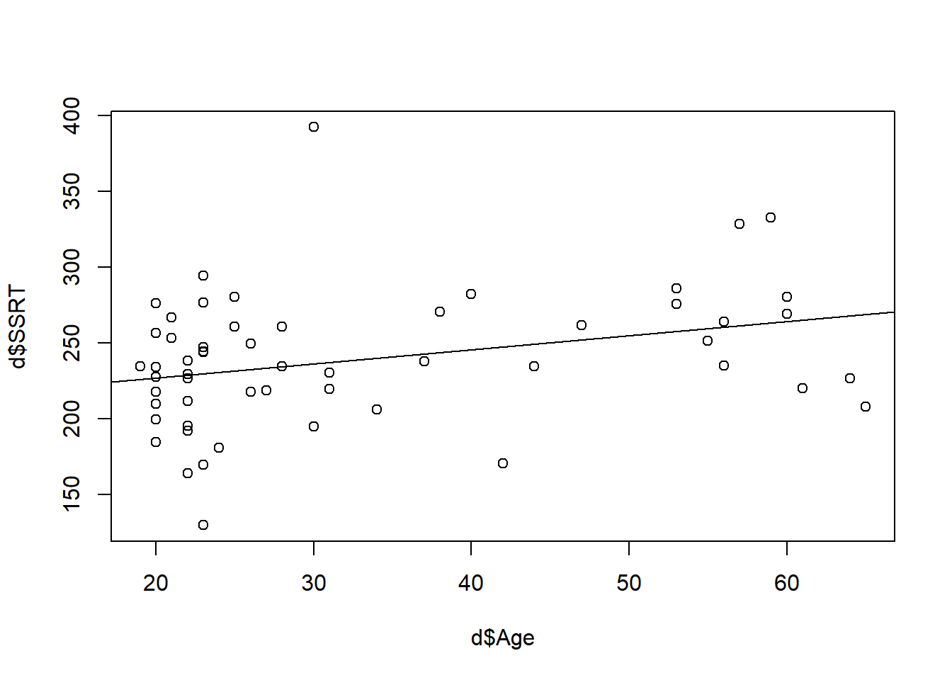
## scale(Age) 2.449481 25.17552The confidence interval for \(\beta_1\) is about 2 to about 25. This means that although we are not sure about the absolute value of \(\beta_1\), we are pretty sure it is positive. Given this confidence interval, it is very unlikely that \(\beta_1\) is zero or negative. In other words, we feel somewhat confident that SSRT does increase with age; maybe by 2 msec per 15 years, maybe by 25 msec per 15 years, but probably not by 0, -10, or 50 msec per 15 years.
A scatterplot of SSRT by age seems to bear this out (I have added a line of best fit to make the point)
6.5 Statistical significance: The bit about p-values
You will have noticed that the final column in the summary of m2 contains something called the p-value (Pr(>|t|)). This may or may not have some exciting asterisks ** next to it. I mentioned earlier that the General Linear Model provides us with parameter estimates and their precision; but also with statistical tests. In particular, it provides us with a statistical test of the hypothesis that the parameter in question might be zero. Generally, when the p-value is smaller than a critical value (often taken as 0.05), the result is regarded as statistically significant, and the null hypothesis that the parameter could be zero is considered rejected on the basis of the evidence.
The p-value is sometimes described as something like ‘the probability that the result is due to chance’ or ‘the probability that the null hypothesis is true’. This is in fact an incorrect definition; we don’t know the probability that the null hypothesis is true and cannot estimate that without information that we do not have. Rather than the probability the null hypothesis is true given the data, the p-value actually reflects the probability of observing data this extreme given that the null hypothesis is true. If you have studied the mathematics of Bayes rule, you will know that the probability of the hypothesis given the data is not the same thing as the probability of the data given the hypothesis. You can have a very very small p-value and the null hypothesis still be true. For many, or even most, published results with small p-values, and hence where the researchers have concluded that the result is ‘statistically significant’, the null hypothesis is in fact true (Ioannidis 2005). This is why many published effects in cognitive science do not replicate (Open Science Collaboration 2015).
People in cognitive science get very excited about significant p-values, but I would like to encourage you not to get too hung up on them, and consider parameter estimates and their precision as more important. The magnitude of the parameter estimate is known as the effect size. The reasons I would urge you to think more about effect sizes than p-values are the following:
Because the size of the p-value depends heavily on sample size. In a very small sample, almost no effects or associations will be ‘significant’ (because the precision of the parameter estimates will be low). In a huge sample, almost all of them will be significant (since there is very rarely exactly zero association between two things, and the precision of your estimates is very high in a large sample). So the p-value does in itself not tell you which associations are important. The effect size is, by contrast, independent of sample size, although the precision of your estimate of it does improve with a larger sample.
Because actual scientific questions are usually about effect sizes, not p-values. For example, if I study the effectiveness of psychotherapy, my question is probably not ‘is the effect of psychotherapy on mental health exactly zero?’. It is unlikely that sitting with a sympathetic listener for an hour a week makes exactly zero difference, on average, to how people feel. My question is probably something like ‘how big is the effect of psychotherapy of mental health?’. Only by answering this latter question could I compare the effect of psychotherapy to those of other treatments; or figure out if the benefit of psychotherapy is worth the cost. Hypotheses are mostly not about the existence of some effect, but about its magnitude and direction.
Because, as already mentioned, you can get plenty of significant p-values, especially if you set the threshold at 0.05, even when the null hypothesis is true. If you run enough statistical tests, some of them will be significant. In particular, with the threshold at p = 0.05, one in twenty tests will be significant, but this does not mean that that effect will generalize to a new sample. With any reasonably complex dataset, there may be dozens of tests you could run, so we should not get too excited if a few of them are significant. This means that p-values become problematic when your research is exploratory rather than confirmatory, and it is also the reason why it is essential to pre-register which predictions you really made prior to data analysis, and try to keep the number of statistical tests as few as possible.
6.6 Summary
In this practical, we have:
learned to fit a General Linear Model with a binary predictor variable;
learned to fit a General Linear Model with a continuous predictor variable;
learned to interpret parameter estimates and their confidence intervals;
encountered statistical significance and had a homily on why not to get too fixated on it.