Chapter 14 Understanding Probablity
14.1 Definitions
Probability is the branch of mathematics that is concerned with assigned the likelihood of the occurrence of an event.
We often use formal and informal assessments of probability in everyday life. For example, you may check the weather before going to work to see the chance of rain, as predicted by meteorologists. Alternatively, you might just look out the window and determine for yourself if rain is likely or unlikely.
experiment: Broadly defined as any activity that we can observe where the result is a random event.
outcome: one out of the many potential results of a random process (Examples: It rains tomorrow; I flip a coin and get ‘heads’; I roll two dice and get a total of 7; I ask a student what year of school they are in and they say ‘Freshman’)
event: A set of one or more of these outcomes. Typically denoted with letters at the beginning of the alphabet.
examples: \(A=\{heads\}\), \(B=\{7,11\}\), \(C=\{all \: freshaman \: and \: sophomores \}\)
The probability of an event is the relative likelihood of an event, which is \(0 \leq A \leq 1\). For \(P(A)=0\), the event must be impossible (i.e. the sum of 2 dice is equal to 1). For \(P(A)=1\), the event must be sure to happen (i.e. the sum of 2 dice is an integer). Values close to zero indicate an event unlikely to happen, while probabilities close to one indicate an event that is likely to happen.
We will spend a fair amount of time discussing how these probabilities are assigned.
14.2 Personal (Subjective) Probability
There are several methods for assigning the numerical values to the probability of an event occurring. If the event is based upon an experiment that cannot be repeated, we use the personal or subjective approach to probability.
Suppose I define event \(A\) to be the likelihood that it will rain today and I wish to know \(P(A)\). How can this be determined? Well, we could do a variety of things:
Look back on data from previous years on how often it rains on this date
Consult a weatherman (i.e. find the forecast on TV, radio, online)
Ask the old man who claims that if his knee aches, that means it is about to rain.
While some of these methods are more scientific than others (i.e. professional meteorologists have advanced climate models to use in assigning thes probabilities), this is based on an experiment which cannot be repeated, since we will observe and live through tomorrow only once. Maybe you remember the movie Groundhog Day or episodes of Star Trek: The Next Generation where the same day was repeated many times, but that doesn’t actually happen.
In class, I asked you to look up on your phone the ‘chance’ of rain in Murray today. Depending on where you looked it up, the percentage given was not always the same. Similarly, if I ask you what is the probability the St. Louis Cardinals win the World Series of baseball next year, I will get different answers. These answers depend on both one’s expertise and one’s bias (i.e. you might not follow baseball and have no idea or you might be a huge Cardinals fan and over-estimate the probability).
As an another example, we are interested in the probability that a patient who has just received a kidney transplant will survive for one year. This patient will only go through the next calendar year once, and will either survive or die. If the subjective probability is assigned by an expert, such as the patient’s surgeon, it might be fairly accurate.
However, subjective probability can be flawed if the probability is assigned by someone who is not an expert or is biased. If I am assigning the probability of the Chicago Cubs winning the World Series next year as \(P(C)=0.75\) (i.e. 75%), you could question both my baseball knowledge (or lack thereof) and my bias (I am a Cubs fan). For this reason, we try to avoid the subjective approach when possible.
14.3 Objective Probability
When we assign a numerical value to the probability of an event that CAN be repeated, we obtain an objective probability.
As the simplest type of experiment that can be repeated, consider flipping a coin, where event \(H\) is the probability of obtaining ‘heads’. I know you already know the answer to the question ‘What is \(P(H)\)?’, but suppose you are a Martian and have never encountered this strange object called a ‘coin’ before.
Our friendly Martian decides to conduct a simulation to determine \(P(H)\) by flipping the coin a large number of times. Suppose the Martian flips the coin 10,000 times and obtains 5,024 heads. His estimate of the probability is
\[ \begin{aligned} P(H) & = \frac{\text{number of occurrences of event}}{\text{total number of trials}} \\ P(H) & = \frac{5024}{10000} = 0.5024 \\ \end{aligned} \]
This is called the empirical or the relative frequency approach to probability. It is useful when the experiment can be simulated many, many times, especially when the mathematics for computing the exact probability is difficult or impossible.
14.4 Law of Large Numbers
The mathematician John Kerrich actually performed such an experiment when he was being held as a prisoner during World War II.
This example illustrates the Law of Large Numbers, where the relative frequency probability will get closer and closer to the true theoretical probability as the number of trials increase.
For instance, if I flipped a coin ten times and got 7 heads, you wouldn’t think anything was unusual, but if I flipped it 10,000 times and got heads 7,000 times, you would question the assumption that the coin was “fair” and the outcomes (heads or tails) were equally likely.
14.5 Classical Probability
The other type of objective probability is called classical probability, where we use mathematics to compute the exact probability without actually performing the experiment.
For example, we can determine \(P(H)\) without ever flipping a coin. We know there are two possible outcomes (heads and tails). If we are willing to assume the probability of each outcome is equally likely (i.e. a “fair” coin), then \(P(H)=\frac{1}{2}\).
Similarly, if we roll a single 6-sided die and let event \(A\) be the event that the die is less than 5, then notice that 4 of the 6 equally likely events contain our desired outcome, so \(P(A)=\frac{4}{6}\).
Clever mathematics, which can get quite difficult, can be used to compute probabilities of events such as the probability of getting a certain type of hand in a poker game or winning the jackpot in a lottery game such as Powerball.
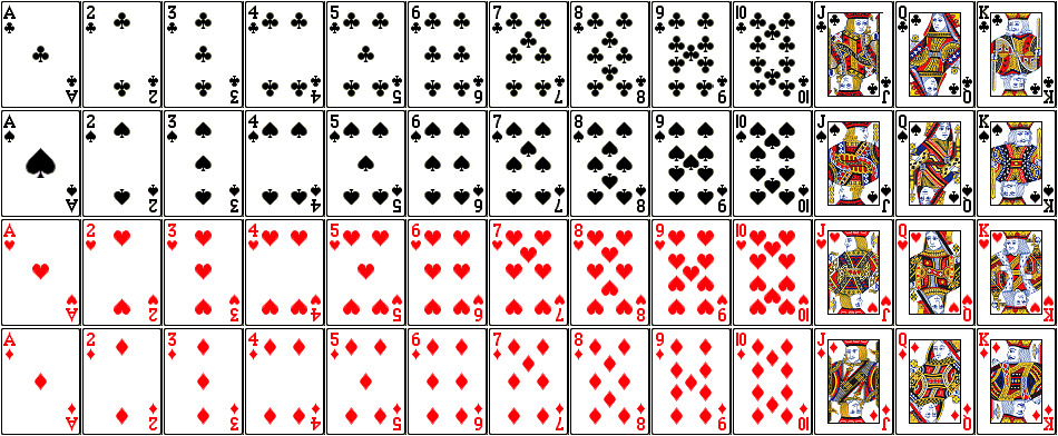
14.6 The Deck of Cards
A standard deck of cards contains 52 cards. The cards are divided into 4 suits (spades, hearts, diamonds, clubs), where the spades and clubs are traditionally black and the hearts and diamonds are red. The deck is also divided into 13 ranks (2, 3, 4, 5, 6, 7, 8, 9, 10, Jack, Queen, King, Ace). The Jack, Queen, King are traditionally called face cards. The Ace can count as the highest and/or lowest ranking card, depending on the particular card game being played.
14.7 Probabilities from Cards
A player receives one card, at random, from the deck. Let \(A\) be the event the card is an Ace, \(B\) that the card is a heart, and \(C\) that the card is a face card.
\[P(A)=\frac{4}{52}=\frac{1}{13}\]
\[P(B)=\frac{13}{52}=\frac{1}{4}\]
\[P(C)=\frac{4+4+4}{52}=\frac{12}{52}\]
\[P(A \: and \: B)=\frac{4}{52}+\frac{13}{52}-\frac{1}{52}=\frac{16}{52}\]
\[P(A \: and \: C)=\frac{0}{52}=0\]
14.8 Blood Type Problem
Suppose everyone in the population has one and exactly one of the four basic blood types (O, A, B, and AB). This is an example of mutually exclusive evnets. Notice, we are not considering the Rh factor \(+\) or \(-\) in this problem.
The percentages in the table below are roughly true for the US population. These probabilities will fluctuate for different countries, as certain blood types are more or less common among certain ethnic groups.
| Blood Type | Probability |
|---|---|
| Type O | 0.45 |
| Type A | 0.40 |
| Type B | 0.11 |
| Type AB | ? |
Suppose I choose one person at random:
\(P(AB)=1-(.45+.40+.11)=1-.96=.04\) or about 4% have Type AB blood.
\(P(A \: or B) = .40 + .11 = .51\) or about 51% have either Type A or Type B blood.
\(P(not O)=P(O^c)=1-P(O)=1-.45=.55\), or about 55% do not have Type O blood.
Suppose I choose three people at random, in such a way as the people are independent (i.e. everone’s blood type does not depend on the others, so we wouldn’t want to choose people who are related)
\(P(all \: 3 \: are \: Type \: O) = .45 \times .45 \times .45 = (.45)^3\)
\(P(none \: have \: Type \: AB) = (1-.04)^3 = (.96)^3\)
\(P(at \: least \: one \: is \: Type \: B) = ???\)
The last problem is easier if we find the probability of the complement (the opposite is the probability that none have Type B), and subtract that probability from one.
\(P(at \: least \: one \: is \: Type \: B) = 1 - (1-.11)^3 = 1-(.89)^3\)
14.9 Addition Rule
Suppose event \(A\) is the event that a middle-aged person has hypertension and event \(B\) is the event that they have high cholesterol. Obviously a person could have both of these conditions; in other words, events \(A\) and \(B\) are NOT mutually exclusive.
Suppose we know that \(P(A)=0.34\), \(P(B)=0.45\), and \(P(A \: and \: B)=0.24\), where \(A \: and \: B\), sometimes written \(A \cap B\) is the intersection, or the probability of event A AND event B (i.e. having both hypertension and high cholesterol).
We want to know \(P(A \: or \: B)\), sometimes written \(A \cup B\), the intersection, or the probability of event A OR event B. The addition rule states:
\[P(A \: or \: B)=P(A)+P(B)-P(A \: and \: B)\]
In our medical example, \[P(A \: or \: B)=0.34+0.45-0.24=0.55\]
We subtract the probability of the intersection to correct for the fact that we would ‘double count’ those individuals with both hypertension and high cholesterol if we did not.
If events \(A\) and \(B\) are mutually exclusive, then \(P(A \: and \: B)=0\).

14.10 Complement Rule
The complement of an event is the probability of all outcomes that are NOT in that event. For example, if \(A\) is the probability of hypertension, where \(P(A)=0.34\), then the complement rule is: \[P(A^c)=1-P(A)\]
In our example, \(P(A^c)=1-0.34=0.66\). This may seen very simple and obvious, but the complement rule can often save a lot of work, in situations where finding the probability of an event is difficult or impossible but the probability of its complement is relatively easy to find.
14.11 Multiplication Rule
The multiplication rule is used to find the probability of an intersection \(P(A \cap B)\), or \(A\) AND \(B\).
When the events are independent,
\[P(A \: and \: B)=P(A) \times P(B)\]
14.12 Coin Flipping (independent)
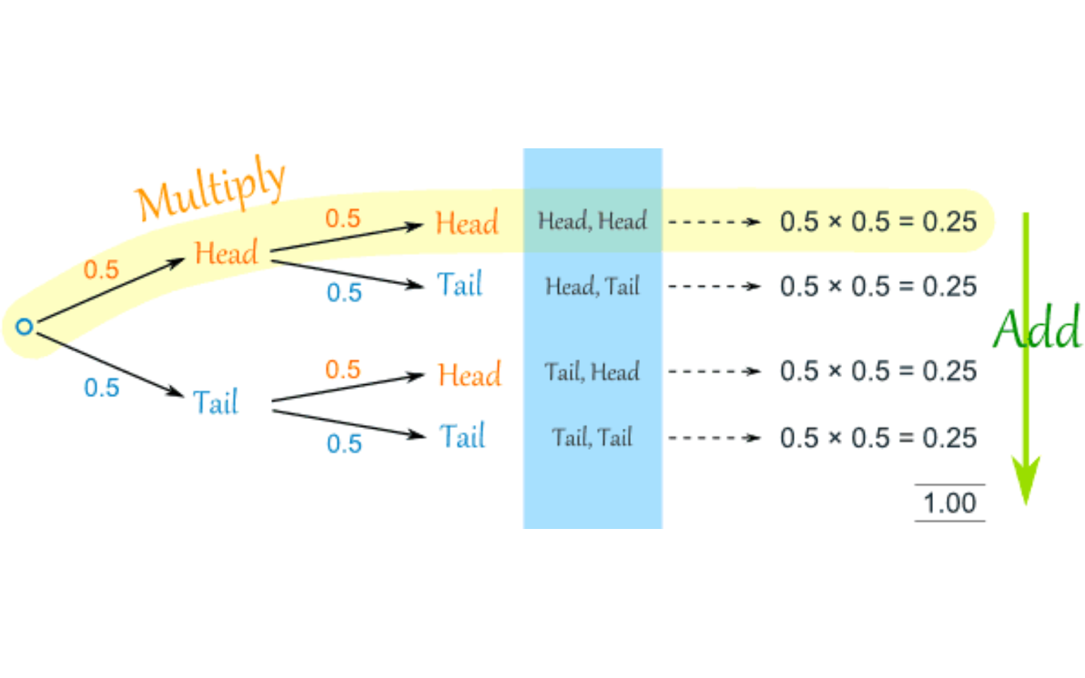
Let \(H_1\) represent flipping a coin and getting heads. Let \(H_2\) represent flipping a second coin and getting heads. It is known that \(P(H_1)=\frac{1}{2}\) and that \(P(H_2)=\frac{1}{2}\).
How can we find the probability that both events occur, i.e. \(P(H_1 \quad and \quad H_2)\)? How about exactly one of the two events? Neither of the two events?
We’ll use the multiplication rule and construct a tree diagram.
The probability of both events is: \[P(H_1 \quad and \quad H_2)=P(H_1)\times P(H_2)=\frac{1}{2} \times \frac{1}{2}=\frac{1}{4}\].
14.13 Expected Value
Consider the following probability distribution table, where \(X\) is the score on the AP Stats exam and \(P(X)\) is the probability of a student receiving that score. The probabilities in this example were found using relative frequency (i.e. counting how many students got each score), not with a mathematical function.
As many of you know, AP exams are scored on a 1 to 5 scale, so there are exactly 5 possible values for \(X\).
| \(X\) | \(P(X)\) |
|---|---|
| 1 | 0.15 |
| 2 | 0.20 |
| 3 | 0.35 |
| 4 | 0.20 |
| 5 | ??? |
We know that all probabilities must be between 0 and 1 (or 0% to 100%). We also know that the probabilities of all possible value of \(X\) sum to 1 (100%), i.e. \(\sum P(X=x) = 1\).
My cousin went to Notre Dame, which would only accept an AP score of \(X=5\) for credit in their classes. We can find the missing probability:
\[P(X=5)= 1-(0.15+0.20+0.35+0.20) = 1-0.90=0.10\]
At Murray State, we typically accept a score of 3 or higher in order to grant credit for the AP course.
\[P(X \geq 3)=P(X=3)+P(X=4)+P(X=5)=0.35+0.20+0.10=0.65\]
Suppose we changed our policy and would only accept scores greater than 3.
\[P(X > 3)=P(X=4)+P(X=5)=0.20+0.10=0.30\]
The expected value (mean) of any discrete probability distribution can be computed as: \[\mu_X=E(X)=\sum x \times P(X=x)\]
\[\mu_X=E(X)=1(0.15)+2(0.20)+3(0.35)+4(0.20)+5(0.1)=2.9\]
14.14 Expected Value of a Casino Game
One of the more basic casino games is roulette. One wager that can be made is to pick your ‘lucky’ number between \(1,2,\cdots,35,36\). Suppose ‘27’ is my lucky number and I wager one matchstick ($1) on ‘27’. I will be paid 35-to-1 and win $35 (35 matchsticks) if the number ‘27’ comes up when the wheel is spun and the ball drops into that slot.
If there are 36 numbered slots from \(1,2,\cdots,35,36\) and each slot is equall likely, we can compute the expected value of the game.
| Outcome | \(X\) | \(P(X)\) |
|---|---|---|
| Win | 35 | \(\frac{1}{36}\) |
| Lose | -1 | \(\frac{35}{36}\) |
\[E(X)=35 \times \frac{1}{36} + -1 \times \frac{35}{36}=\frac{35}{36}-\frac{35}{36}=0\]
When the expected value of a game is zero, it is said to be a fair game. Over the long run, we would expect to break even.
Obviously, casinos do not generally offer fair games, as they want to make a profit and they have expenses. In the actual game of roulette, there are actually 38 numbered slots, 1 through 36 and also ‘0’ and ‘00’, but you are still paid 35-to-1 for a win as if there were only 36 numbered slots.
| Outcome | \(X\) | \(P(X)\) |
|---|---|---|
| Win | 35 | \(\frac{1}{38}\) |
| Lose | -1 | \(\frac{37}{38}\) |
\[E(X)=35 \times \frac{1}{38} + -1 \times \frac{37}{38}=\frac{35}{38}-\frac{37}{38}=\frac{-2}{38}=-0.053\]
For every $1 or matchstick wagered, you expect to lose about $0.053. The ‘house edge’ is 5.3%.
14.15 Expected Value of Insurance
Insurance companies employ analysts known as actuaries, whose job is to evaluate risk and help the insurance companies determine how much to charge for premiums that they sell. Let’s consider a very simplified insurance scenario.
When I worked as a seasonal worker in Yellowstone National Park when I was a student, the seasonal workers all had an insurance policy (there was a small deduction from our paycheck for this policy) that would pay me (or my next-of-kin) a fixed amount if I were killed or disabled during the summer. A challenge for the actuaries is to accurately find the probabilities of events such as death, etc.
| Outcome | \(X\) | \(P(X)\) |
|---|---|---|
| Death | $10000 | 0.001 |
| Disability | $5000 | 0.002 |
| Neither | 0 | 0.997 |
\[E(X)=10000 \times 0.001 + 5000 \times 0.002 + 0 \times 0.997 = 20\]
The insurance company would need to charge more than $20 for this policy in order to expect a profit.
If your neighbor offered you $100 per year to insure his home, where you would have to pay to rebuild his home if it were destroyed in a fire but otherwise could keep the $100, would you do so?
Most people say ‘NO WAY’, because the risk of having to pay many thousands of dollars to rebuild the neighbor’s home is too much to take, and is not worth $100 to you. Insurance companies take on this risk for thousands of customers, and recoup the money paid out with the premiums collected from those of us that do not file a claim.
14.16 Let’s Make a Deal
This is a pretty well-known problem, based on the game show Let’s Make a Deal. It is sometimes called the Monte Hall problem, after the host of the show back in the 1960s and 1970s.
There are three doors; behind one is a prize (say a car or lots of money which you want), and behind the other two is no prize (or something you don’t want). You choose a door, and the game show host shows you one of the doors you didn’t choose, where there is no prize. The host (Monte Hall or Wayne Brady) offers you a chance to switch to the other unopened door.
  1. Should you switch doors?

  2. Should you stay with your first choice?

  3. Maybe it doesn't matter and you could just flip a coin...
If you saw the TV show ‘Numb3rs’ or the movie ‘Twenty-One’, the problem was featured:
You can simulate the game here:
Why is it better for you to switch your choice than stay with your initial guess? (You might draw a tree diagram to see why)
Suppose you chose Door #1. The game show host shows you that there was a “goat” behind Door #3, but instead of giving you the option to switch to Door #2 (which we now know is the best option), he offers us $1000 to give up the door. If the car is worth $24,000, what is the expected value of keeping the door and turning down the cash?
| Outcome | \(X\) | \(P(X)\) |
|---|---|---|
| Car | $24000 | \(\frac{1}{3}\) |
| Goat | $0 | \(\frac{2}{3}\) |
\[E(X)=24000 \times \frac{1}{3} + 0 \times \frac{2}{3} = 8000\]
We see that from a purely mathematical aspect, we should turn down the $1000 and keep our “equity” with the door, even though most of the time we will lose.
Obviously from a psychological standpoint and from a practical standpoint, the higher the offer, the more likely most people are to take the “sure thing”. None of you were interested in an offer of $1 if the prize was a $24 gift certificate to a local restaurant.
People with high risk aversion are likely to take even small offers well below the expected value, whereas people with low risk aversion are likely to “gamble” and to try to win the big prize, even if the offer exceeds the expected value.
This can be rigorously quantified in economic theory with the utility function: a mathematical function that ranks alternatives according to their utility to an individual.