Chapter 11 Linear Regression
11.1 Guessing the Line of Best Fit
Data Set: Variable \(X\) is ACT composite score; the \(X\) variable will be referred to as the explanatory variable, predictor variable, or independent variable
Variable \(Y\) is the freshman college GPA; the \(Y\) variable will be referred to as the response variable or dependent variable
In statistic, we often want to know if two variables \(X\) and \(Y\) are mathematically related to each other, and eventually if we can form a mathematical model to explain or predict variable \(Y\) based on variable \(X\)
This is our same sample of \(n=10\) college students. I have computed the means and standard deviations of both variables.
| \(X\) | \(Y\) |
|---|---|
| 32 | 4.0 |
| 28 | 3.5 |
| 26 | 1.2 |
| 24 | 3.3 |
| 22 | 3.0 |
| 21 | 2.8 |
| 20 | 2.6 |
| 20 | 2.1 |
| 19 | 3.5 |
| 18 | 2.4 |
## [1] "Variable X (ACT Score)"## mean sd
## 23 4.472136## [1] "Variable Y (GPA)"## mean sd
## 2.84 0.8126773## [1] "Correlation between X and Y"## [1] 0.358Below is a scatterplot where we are attempting to “guess” the line of best fit.
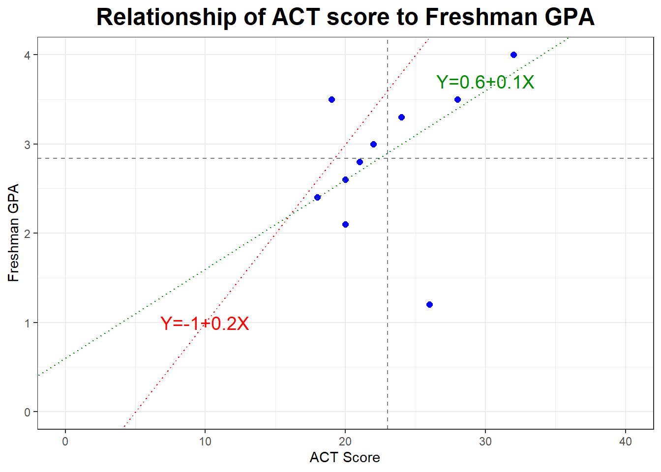 Obviously we aren’t going to actually find the equation for a statistical model by guessing and using trial and error. We need to have some sort of mathematical method of selecting and computing the equation of the “line of best fit”.
11.2 Finding the Line of Best Fit
The equation of this line will be \[\hat{Y}= a + b X\]
Sometimes we just use the actual names of the variables. \[\hat{GPA} = a + b \times ACT\]
\(X\) is the value of our explanatory or independent variable (a student’s score on the ACT in this example)
\(\hat{Y}\) (“y-hat”) is the predicted value of our response or dependent variable (predicted GPA in this case). Suppose your younger sibling is in high school and got \(X=25\) on the ACT; we could use the regression model to predict their GPA, and denote this prediction with \(\hat{Y}\). When they actually come to college, their actual GPA will be \(Y\) (without the hat).
\(b\) is the slope of the regression line and \(a\) is the \(y\)-intercept of the line. You probably used \[y=mx+b\] in high school with \(m\) for slope and \(b\) for the \(y\)-intercept.
In order to estimate the numerical values of the slope and intercept \(b\) and \(a\), we use a mathematical criterion called least squares estimation. We choose the line whose equation will minimize the sum of squared residuals.
What’s a residual? A residual is the vertical distance between an actual observed data point and the predicted point. You can think of it as the “error” in our prediction, and we use the letter \(e\) for it.
\[e=Y-\hat{Y}\]
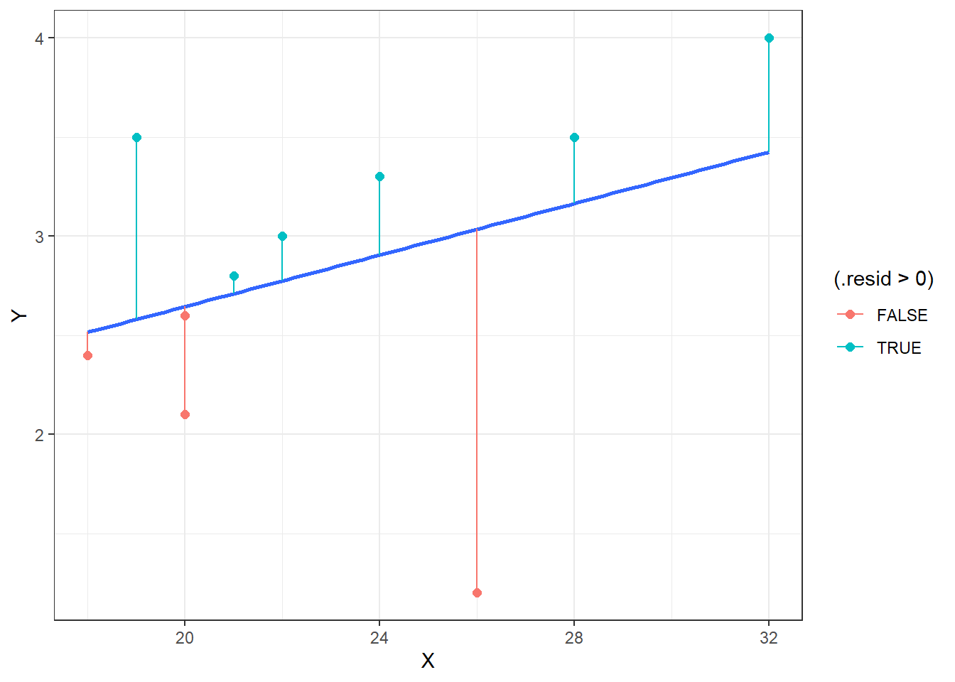 The largest positive residual was for student #9 (\(X=19,Y=3.5\)). This is the point the furtherest above the blue least squares regression line, as this student’s actual GPA was much higher than the model predicted.
On the other hand, student #3 (\(X=26,Y=1.2\)) had the largest negative residual. This student did much worse than predicted.
Some students have points very close to the line. These residuals are equal to almost zero, indicating that the actual GPA \(Y\) and the predicted GPA \(\hat{Y}\) are very close.
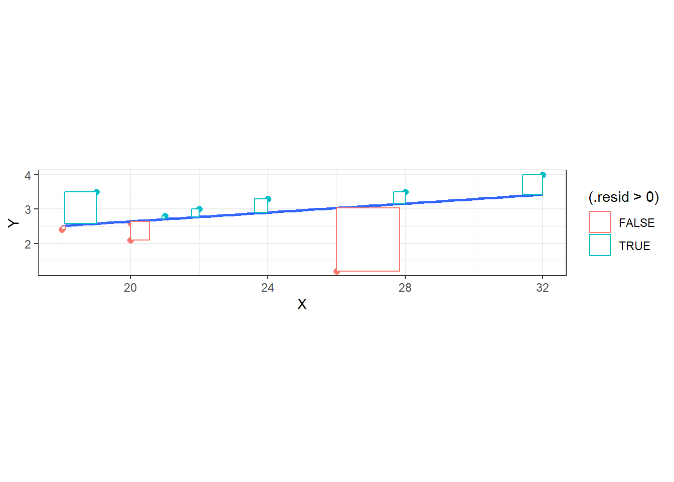
If we square and sum the residuals for all points, we obtain the sum of squared residuals \[SSR = \sum_{i=1}^n (Y_i - \hat{Y_i})^2\]
The blue least squares regression line is the one that minimizes \(SSR\), represented below as the area of the rectangles. No other line would make the area of those rectangles smaller.
Through the use of calculus, the equations for the least squares regression line are: \[b = r \frac{s_Y}{s_X}\]
\[a = \bar{Y} - b \bar{X}\]
For the GPA-ACT example, we get:
\[b = 0.3577 \times \frac{0.8127}{4.4721} = 0.0650\]
\[a = 2.84 - 0.0650 \times 23 = 1.3450\]
Thus, the least squares regression model has the following equation:
\[\hat{Y}=1.345 + 0.065X\]
11.3 Interpreting the Regression Model
What do the numerical values of \(a\) and \(b\) physically represent?
\(a\) is the \(y\)-intercept, the predicted value of \(Y\) when \(X=0\). In our case, our model predicts a GPA of 1.345 when the ACT score is 0, which doesn’t make sense in this context.
It is pretty common for the \(y\)-intercept to have no physical meaning; this happens when \(X\) will never be equal to 0. If we were trying to predict the gas mileage of a car based on its weight, no car weighs \(X=0\) pounds. However, if we are trying to predict the ozone level based on wind speed, a day with no wind would have \(X=0\), and in that case the intercept of the regression equation is the predicted ozone level on a day with no wind.
\(b\) is the slope, or the rate of change. It tells us the predicted increase/decrease in \(Y\) with a one unit increase in \(X\). Note that the slope of the regression equation will always have the same sign as the correlation between \(X\) and \(Y\). In our example, \(b=0.065\) means that we predict the GPA will increase by 0.065 for every 1 point increase in the ACT score.
Suppose we try to predict the GPA for a student with an ACT score of \(X=26\).
\[\hat{Y} = 1.345 + 0.065 \times 26 = 3.035\]
Student #3 in our data set has \(X=26\) but had a very low GPA of \(Y=1.2\). They have a large residual
\[e = Y - \hat{Y} = 1.2 - 3.035 = -1.835\]
Student #6 had an ACT of \(X=21\) and a GPA of \(Y=2.8\). Notice this student’s predicted GPA is very close to their actual GPA, and the residual is close to zero.
\[\hat{Y} = 1.345 + 0.065 \times 21 = 2.71\]
\[e = 2.8 - 2.71 = 0.09\]
The coefficient of determination, or \(r^2\), is used as a measure of the quality of a regression model. One reason for using this statistic is that the correlation \(r\) is NOT a percentage, but $r^2 is.
\[r^2=(.358)^2=.128\]
The interpretation of \(r^2\) in our example is: About 12.8% of the variation in the freshman GPA is explained by our model that uses ACT score.
As you can see, this result is not terribly impressive, as we want \(r^2\) to be close to 1 (100%). If we delete Student #3 (the influential point), we have a substantial change in the correlation & regression statistics.
## [1] "Mean and Standard Deviation of X, ACT"## mean sd
## 22.66667 4.609772## [1] "Mean and Standard Devaition of Y, GPA"## mean sd
## 3.022222 0.6078194## [1] "Correlation between ACT and GPA"## [1] 0.766## [1] "Intercept and Slope"## (Intercept) X
## 0.7333333 0.1009804## `geom_smooth()` using formula = 'y ~ x'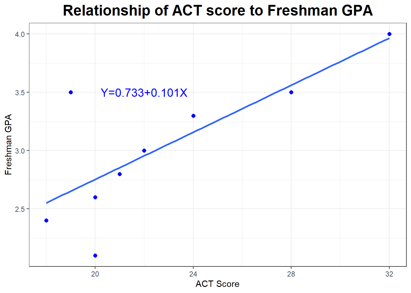
Now the regression model is \[\hat{Y}=0.733 + 0.101 X\] with \(r=.766\) and \(r^2=.587\), indicating that about 58.7% of the variation in GPA is explained by the model using ACT score,
11.4 Dangers of Extrapolation
Indiscriminate use of regression can yield predictions that are ridiculous.
The graph and regression line below show the relationship between the mean height (in cm) and age (in momths) of young children in Kalama, Egypt.
## # A tibble: 12 × 2
##      age height
##    <int>  <dbl>
##  1    18   76.1
##  2    19   77
##  3    20   78.1
##  4    21   78.2
##  5    22   78.8
##  6    23   79.7
##  7    24   79.9
##  8    25   81.1
##  9    26   81.2
## 10    27   81.8
## 11    28   82.8
## 12    29   83.5
##
## Call:
## lm(formula = height ~ age, data = Kalama)
##
## Coefficients:
## (Intercept) age
## 64.928 0.635## `geom_smooth()` using formula = 'y ~ x'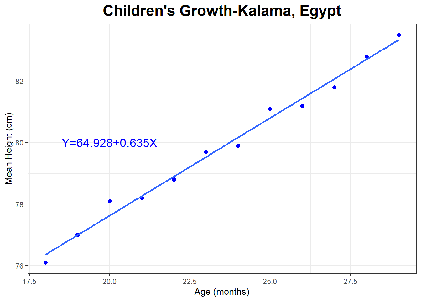
Let’s predict the height of a 50 year old man.
\[X=50 \times 12 = 600\]
\[\hat{Y}=64.928 + 0.635 \times 600 \approx 446\]
The man is predicted to be about 446 cm, or 4.46 m tall. Divide cm by 2.54, the predicted height is about 176 inches tall, or about 14 feet 8 inches tall.
This is obviously a terrible prediction, even though \(r^2=.989\) for the model . Think about how humans tend to grow and what the linear regression model is assuming about how we grow.