Chapter 19 Sampling Distributions

19.1 Rule For Sample Proportions

Suppose we have a population with a fixed proportion of success, which we denote as the parameter \(p\). We are able to draw a random sample from this population.

If the sample is ‘large’ enough with both \(np>10\) and \(n(1-p)>10\) (i.e. expected number of successes and failures are at least 10), then \(\hat{p}\) will be approximately normal.

\[\hat{p} \dot{\sim} N(p,\sqrt{\frac{p(1-p)}{n}})\]

Example:

Suppose that a psychic claims to have ESP (extra-sensory perception). A way of testing for ESP is with a special deck of 5 cards, each of which has a different shape.

ESP

With 5 shapes, our chance of guessing correctly on each trial should be \[p=\frac{1} {5}=0.2\]

Suppose we are going to have our psychic guess the shape for \(n=200\) trials, where each trial is independent with the probability of success by guessing is always \(p=0.2\).

The “expected number” of successes for someone guessing randomly is \(np=200(.2)=40\). The “expected number” of failures is \(n(1-p)=200(.8)=160\). Both are much larger than 10 and sufficient for use of the Rule for Sample Proportions.

I will simulate the sampling distribution of the proportion with a computer program.

http://www.lock5stat.com/StatKey/index.html

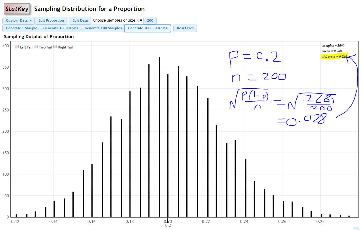
I will choose the option Sampling Distributiond: Proportion, use Edit Proportion to set \(p=0.2\) and set to Choose samples of size \(n=200\).

With the Rule for Sample Proportions, the standard deviation of our proportions (i.e. the standard error) should be (see how close the simulated value for standard error is, along with the shape of the sampling distribution): \[\sqrt{\frac{p(1-p)}{n}} = \sqrt{\frac{0.2(0.8)}{200}} = 0.028\]

19.2 Central Limit Theorem

(your book calls this the Rule For Sample Means, and the Rule For Sample Proportions is a special case): Draw many, many random samples of size \(n\) from some population (which may or may not be normal). If the sample size \(n\) is ‘large’ enough, then the sampling distribution of the sample mean \(\bar{x}\) will be approximately normal.

\[\bar{X} \dot{\sim} N(\mu_{\bar{X}}=\mu, \sigma_{\bar{X}}=\frac{\sigma}{\sqrt{n}})\]

Best Case Scenario (Normal Distribution)

Suppose the amount of liquid, in ML, in a bottle of Diet Pepsi follows a normal distribution \(X \sim(\mu=593, \sigma=1.4)\). Since \(X\) is normal, then \(\bar{X}\) will be normal for any sample size \(n\).

Finding \(P(X<591)\) for a single bottle of Pepsi is just a normal curve problem, solvable with a normal table.

\[Z=\frac{591-593}{1.4}=-1.43\] \[P(X<591)=P(Z<-1.43)=0.0764\]

If we take a sample of \(n=10\) bottles, then \(\sigma_{\bar{x}}=\frac{1.4}{\sqrt{10}}\).

\(Z=\frac{591-592}{1.4/\sqrt{10}}=-4.52\)

\(P(\bar{X}<591)=P(Z<-4.52)\), which is virtually zero.

Worst Case Scenario

If the distribution of \(X\) is unknown or known to be skewed, then \(n \geq 30\) for the sampling distribution to be approx. normal.

Example #1 (Survival Times–Heavily Skewed):

The lifetime of a certain insect could be described by an exponential distribution with mean \(\mu=1000\) hours and standard deviation \(\sigma=1000\) hours. This distribution is heavily skewed and non-normal. This particular continuous distribution is sometimes used to model survival times when deaths/failures happen randomly. More advanced distributions (such as the Weibull) can more accurately model survival when deaths/failures do not occur randomly. When most deaths/failures occur early, an ‘infant-mortality’ model is used, while if most deaths/failures occur later, an ‘old-age wearout’ model is used.

Suppose I want to find \(P(X>1100)\). We cannot (with STA 125 level methods) find this probability, and a normal approximation would be terrible!

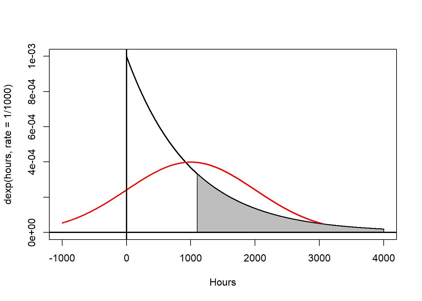
However, using the Central Limit Theorem, we can compute \(P(\bar{X}>1100)\) for a sample of \(n=30\) insects.

I will simulate the sampling distribution and draw its histogram, superimposing a normal curve with mean \(\mu_{\bar{x}}=1000\) and standard error \(\sigma_{\bar{x}}=\frac{1000}{\sqrt{30}}=\) 182.5741858 on top of it.

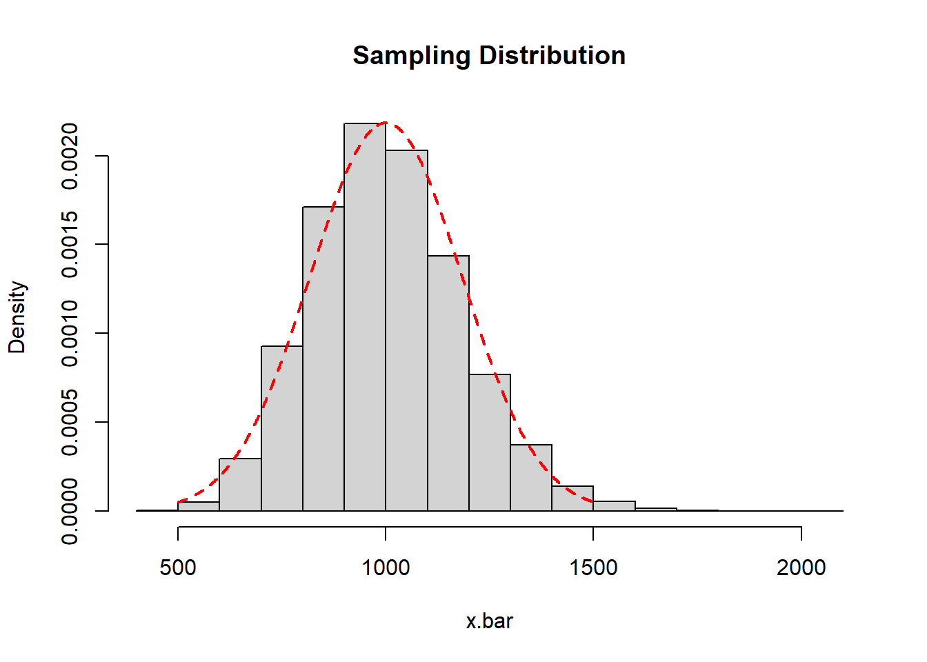
The sample mean of my sampling distribution is 1002.1498714 and the standard deviation of my sampling distribution (standard error) is 182.1122925. these are close to the theoretical values.

So \(P(\bar{X}>1100)\) for a sample of \(n=30\) is just another normal curve problem based on \(\bar{X} \dot{\sim} N(1000,1000/\sqrt{30})\).

\(Z=\frac{\bar{X}-\mu}{\sigma/\sqrt{n}}=\frac{1100-1000}{1000/\sqrt{30}}=\) 0.55

\(P(Z>0.55)=1-0.7088=.2912\)

Example #2 (Baseball Salaries-Heavily Skewed : The beauty of the Central Limit Theorem is that even when we sample from a population whose distribution is either unknown or is known to be some heavily skewed (and very non-normal) distribution, the sampling distribution of the sample mean \(\bar{X}\) is approximately normal when \(n\) is ‘large’ enough. Often \(n > 30\) is used as a Rule of Thumb for when the sampling distribution will be large enough.

A nice online demonstration of this can be found at (http://www.lock5stat.com/statkey/index.html). At this site, go to Sampling Distribution: Mean link (about the middle of the page or directly at http://www.lock5stat.com/statkey/sampling_1_quant/sampling_1_quant.html). In the upper left hand corner, change the data set to Baseball Players-this is salary data for professional baseball players in 2012. On the right hand side, you see that the population is heavily right-skewed due to a handful of players making HUGE salaries.

You can choose samples of various sizes–the default is \(n=10\) and generate thousands of samples. The sample mean \(\bar{X}\) is computed for each sample and the big graph in the middle of the page is the sampling distribution. Notice what happens to the shape of this distribution, along with the mean and the standard error of the sampling distribution.

The original population of \(n=855\) players is heavily skewed and non-normal with mean \(\mu=3.439\) million dollars (wow!) and \(\sigma=4.698\) million. I will take 10000 samples, each of size \(n=50\).

Baseball

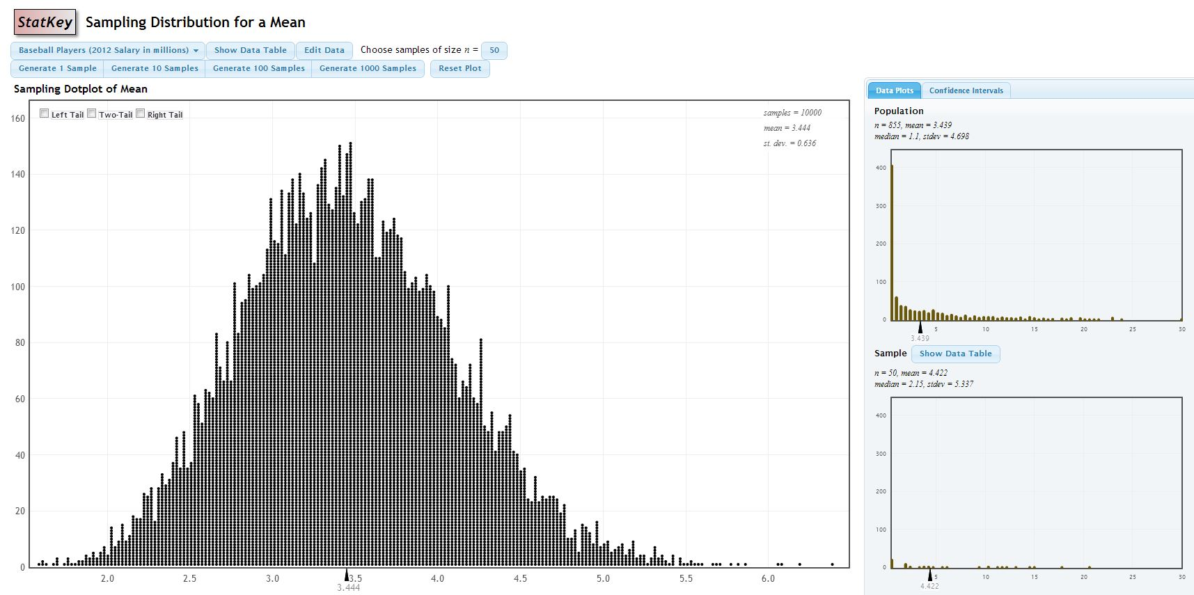
The mean of the sampling distribution of \(\bar{X}\) is \(3.444\), which is very close to \(\mu\) for the population.

The standard error of the sampling distribution is \(0.636\). Theoretically, it should be \(\sigma_{\bar{X}}=\frac{\sigma}{\sqrt{n}}=\frac{4.698}{\sqrt{50}}=0.664\), again very close.

The shape is approximately normal (although a bit of skew is still visible).