Chapter 22 Hypothesis Testing

22.1 One-Proportion \(Z\)-test

In chapter 22, we will study our first example of a hypothesis test, a procedure known as the One-Proportion \(Z\)-test. As you will see, it is closely related to the confidence interval for a proportion \(p\) studied in chapter 20. (Your text covered a hypothesis test called the chi-square test in chapter 13, which we will look at if time allows.)

22.2 Six Step Method for Hypothesis Testing

I will be presenting hypothesis testing via a systematic six step process (your book presents it as a four step process that basically combines my first three steps into one), and will expect you to use these steps when you work problems. I will work through our first example slowly and in great detail, since there is a lot of new concepts and terminology to discuss.

Step One: Write Hypotheses

For our first example, suppose that we have a coin that we suspect is unfair (i.e. the coin will not give us heads 50% of the time if we flip it many times). This research question will be turned into a pair of mathematical statements called the null and alternative hypotheses. Hypotheses are statements about the value of a parameter, not a statistic.

The null hypothesis, or \(H_O\), states that there is no difference (or effect) from the population parameter (hypothesized value) and is what will be statistically tested. The alternative hypothesis, or \(H_A\), states that there is some sort of difference (or effect) from that parameter. The alternative will typically correspond to one’s research hypothesis.

\[H_O: p=0.50\] \[H_A: p \neq 0.50\]

For our artificial first example, the null hypothesis is stating that our coin is fair (gives heads 50% of the time), while the alternative hypothesis is stating that the coin is unfair and does not give heads 50% of the time. This is an example of a two-sided hypothesis, also called a non-directional hypothesis. It is two-sided (non-directional) because we have NOT indicated any sort of a priori belief that the coin was biased to give either more than 50% or fewer than 50% heads when flipped.

In many research situations, we will have a one-sided or directional hypothesis. For example, a medical study might look to see if a treatment will significantly lower the average blood pressure of patients when compared to a control. I will illustrate both possible directions, first if we think the coin is biased in favor of heads.

\[H_O: p=0.50\]

\[H_A: p>0.50\]

Next, consider if we thought the coin was biased in favor of tails.

\[H_O: p=0.50\]

\[H_A: p<0.50\]

Step Two: Choose Level of Significance

This is where you choose your value for \(\alpha\) (usually 0.05), thereby setting the risk one is willing to take of rejecting the null hypothesis when it is actually true (i.e. declaring that you found a significant effect that in fact does not exist).

\[\alpha=0.05\]

A two-sided hypothesis test at level \(\alpha\) will correspond to a \(100(1-\alpha)\%\) confidence interval.

Step Three: Choose Your Test and Check Assumptions This is where you choose your ‘tool’ (i.e. test) and check the mathematical assumptions of that test to make sure you are using the proper ‘tool’ for the job. For the one-proportion \(z\)-test, the assumptions are:

1. the data is from a random sample
2. the data values are independent
3. the sample size is sufficient to use the normal approximation to the binomial

Checking the first two conditions involves judging whether or not the sampling was done in a random and independent fashion. The third condition can be judged mathematically.

Suppose we plan on flipping the coin \(n=400\) times. These flips will clearly be random and independent. We can check to make sure that both the expected number of successes AND the expected number of failures are at least 10; check that \(np_O \geq 10\) and \(nq_0 \geq 10\). In our example, \(n=400\), \(p_O=0.5\) and \(q_O=1-p_O=1-0.5=0.5\), so we have 200 expected successes and 200 expected failures, more than enough, and we may proceed.

Step Four: Calculate the Test Statistic This is what you thought stats class was all about. You will use a formula (or an appropriate function on a calculator or software package) to compute a test statistic based on observed data. The test statistic for this test is:

\[z = \frac{\hat{p}-p_O}{\sqrt{\frac{p_O q_O}{n}}}\]

Suppose we obtain \(X=215\) heads in \(n=400\) flips, such that \(\hat{p}=\frac{215}{400}=0.5375\). Our test statistic will be:

\[z = \frac{.5375-.5}{\sqrt{\frac{0.5(0.5)}{400}}}=\frac{0.0375}{0.025}=1.5\]

The distribution of this test statistic \(z\) will be \(z \sim N(0,1)\) (i.e. standard normal) WHEN the null hypothesis is true.

Step Five: Make a Statistical Decision This is where you either determine the decision rule (‘old-school’) or compute a \(p\)-value (‘new-school’) and decide whether to reject or fail to reject the null hypothesis.

Step Five: Make a Statistical Decision (via the Decision Rule)

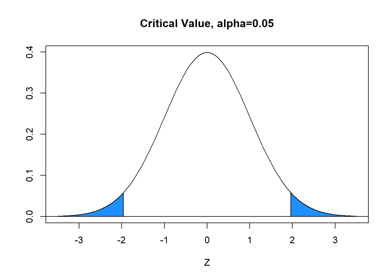
With \(\alpha=0.05\) (area in blue), the critical value is \(z^*=1.96\). The blue tails in the graph below each have area=\(\alpha/2=.025\) and the white area between is equal to \(1-\alpha=0.95\). Hence, the decision rule is to reject \(H_0\) when the absolute value of the computed test statistic \(z\) exceeds critical value \(z^*\), or reject \(H_0\) if \(|z|>z^*\). In our problem, \(|z|=1.50 \not > 1.96=z^*\) and we FAIL TO REJECT the null.

Step Five: Make a Statistical Decision (via the \(p\)-value)

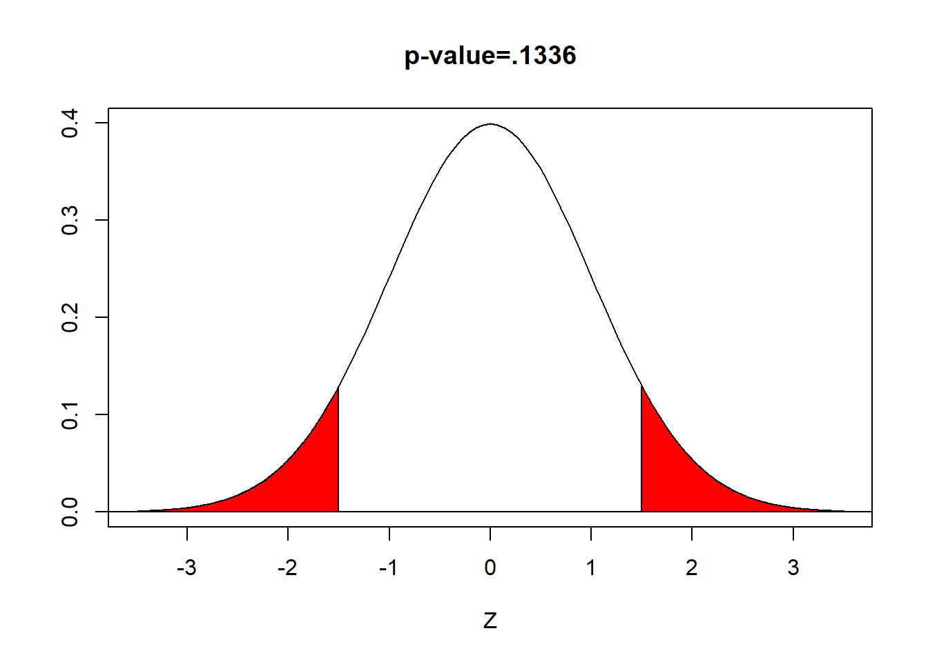
When you use technology, a statistic called the p-value will be computed, based on your computed test statistic. The \(p\)-value is defined to be the probability of obtaining a value as extreme as our test statistic, IF the null hypothesis is true. For our two-sided \(z\)-test,

\[ \begin{aligned} \text{p-value}= & P(|z|>1.50) \\ = & 2 \times P(z<-1.50) \\ = & 2 \times P(z>1.50) \\ = & 2 \times 0.0668 \\ = & 0.1336 \end{aligned} \] (area in red)

• When the \(p\)-value is less than \(\alpha\), we reject the null hypothesis. We have ‘evidence beyond a reasonable doubt’.

• When the \(p\)-value is greater than or equal to \(\alpha\), we fail to reject the null. We do not have ‘evidence beyond a reasonable doubt’.

Here \(.1336>.05\) and we fail to reject the null hypothesis

Step Six: Conclusion This is where you explain what all of this means to your audience. The terminology you use should be appropriate for the audience.

Since we rejected the null hypothesis, a proper conclusion would be:

The proportion of coin flips that are heads is NOT significantly different than 0.50. In other words, we do not have evidence to show the coin is unfair.

Remember, the amount of statistical jargon that you use in your conclusion depends on your audience! If your audience is a committee of professors, you can use more terminology than if your audience is someone like a school principal or hospital administrator or the general public.

22.3 Relationship Between a Two-Sided Test and a CI

In our problem, we computed \(z=1.50\) with \(p=.1336\) and rejected the null hypothesis at \(\alpha=0.05\). Suppose we computed the \(100(1-\alpha)\%\) confidence interval for a proportion for the coin flips data. Here, it is a 95% CI:

\[ 0.5375 \pm 1.96 \times \sqrt{\frac{.5375(1-.5375)}{400}}\] \[0.5375 \pm 0.0489\]

The 95% CI is \((0.4886,0.5864)\). The margin of error is \(\pm 4.89\%\) Notice the confidence interval contains the null value of \(p=0.50\) . This also leads to a failure to reject the null hypothesis (that the coin was fair).

22.4 What if We Have a One-Sided Test?

Suppose your original research hypothesis was that the coin was more likely to land on heads. Step One would change.

\[H_O: p=0.50\]

\[H_A: p > 0.50\]

Steps Two, Three, and Four will not change!

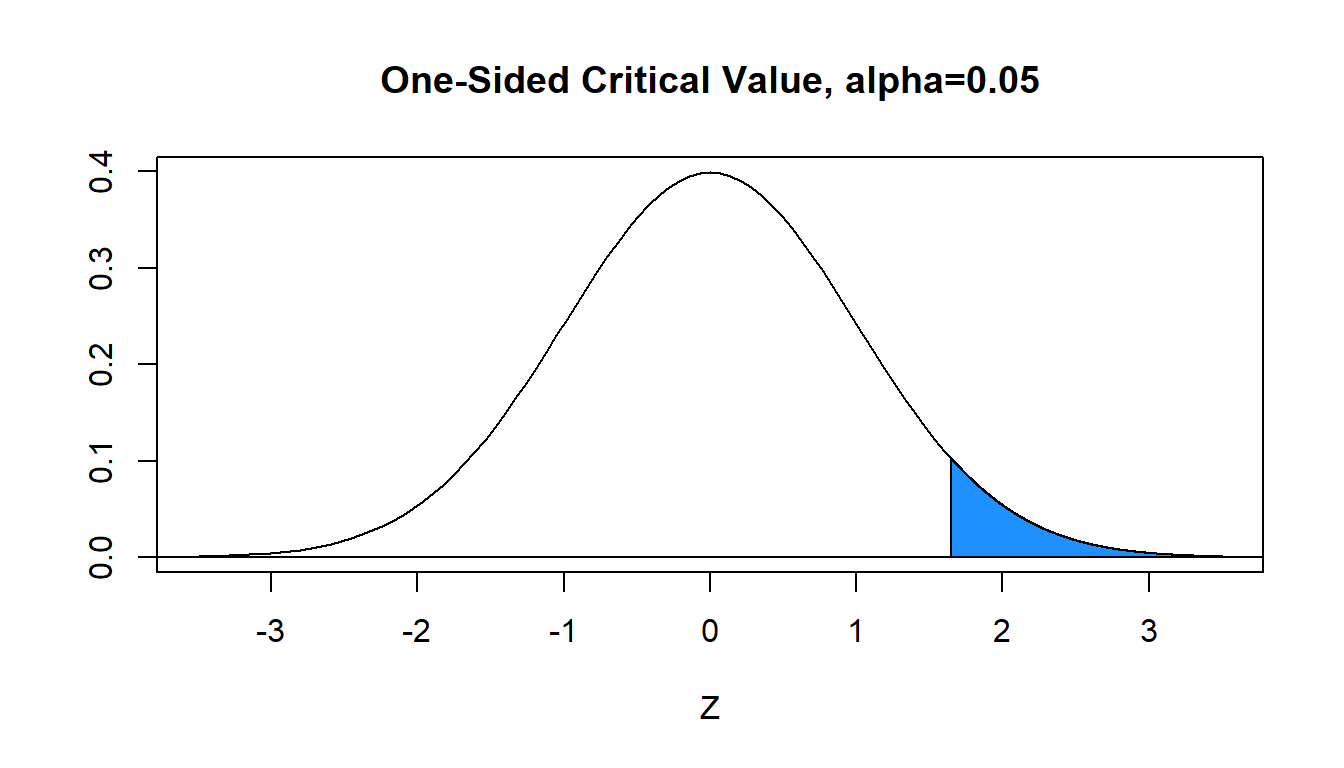
Step Five will change. If you are looking up the critical value \(z^*\) from the table to determine the decision rule, the entire area \(\alpha=.05\) will be on the right (or left) hand side of the normal curve. The critical value is \(z^*=1.645\), so reject \(H_0\) if \(z>1.645\).

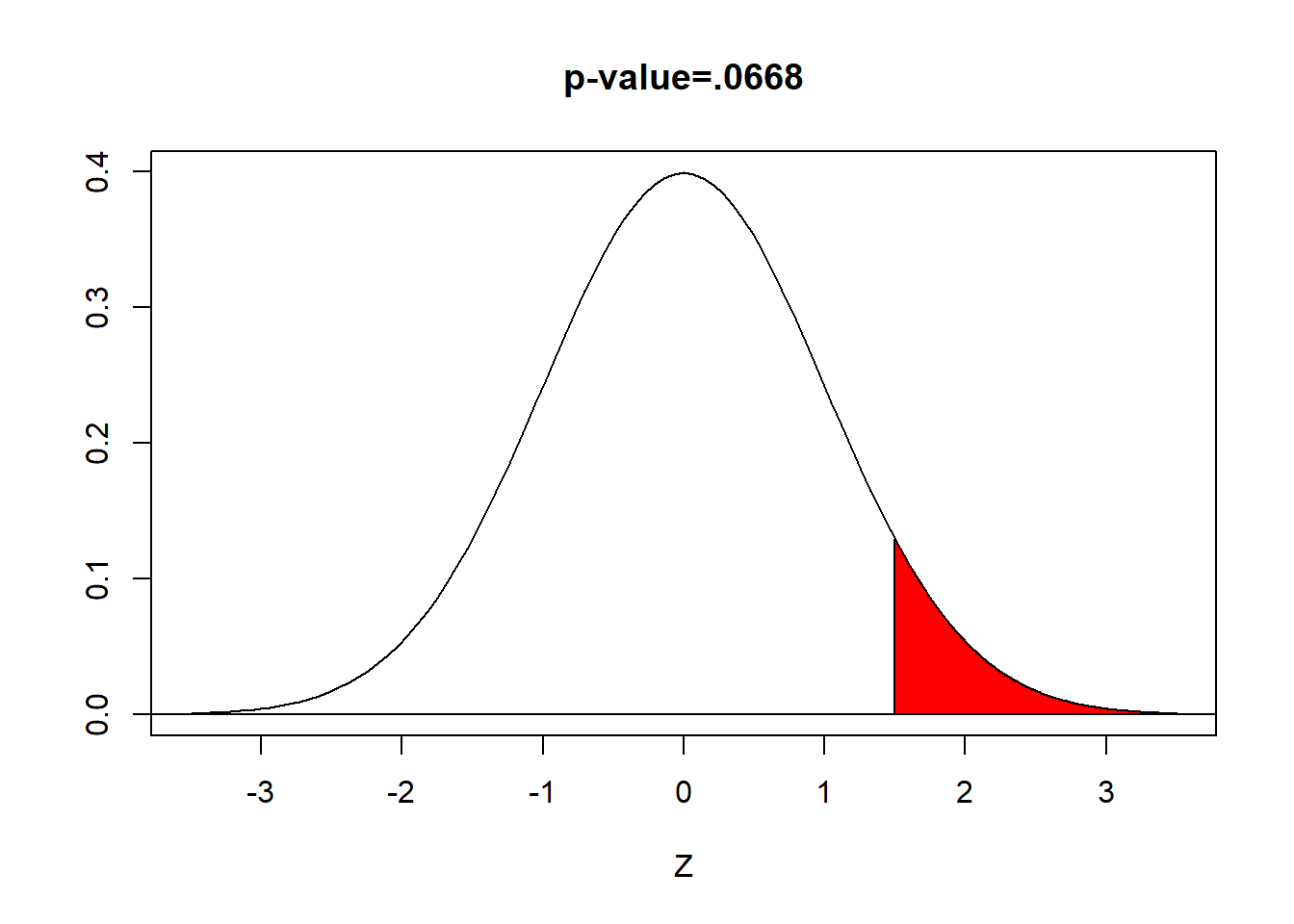
Step Five will change. If you are computing the \(p\)-value, it will only be the area to the right (or left) of the computed test statistic. In our problem, \(\text{p-value}=P(z>1.50)=.0668\). The \(p\)-value will be exactly half of what it was with the two-sided test on the same data.

We still fail to reject; step six will be slightly different:

The proportion of coin flips that are heads is NOT significantly greater than 0.50. In other words, we do not have evidence to show the coin is unfair or biased towards heads.

22.5 The Concept of Hypothesis Testing

The concept behind hypothesis testing is that I first will write a pair of hypotheses \(H_0\) and \(H_a\) that correspond to a research question. Then I collect data via random sampling, choose an appropriate mathematical procedure called a hypothesis test, calculate a test statistic, and decide to either reject the null hypothesis or fail to reject the null hypothesis.

One can draw an analogy between hypothesis testing and a jury trial. The null hypothesis is that the defendant is innocent and the alternative is that he/she is guilty. Evidence is presented during the trial, and the jury decides to either find the defendant guilty (i.e. they rejected the null) or not guilty (i.e. they failed to reject the null due to lack of evidence ‘beyond a reasonable doubt’).

22.6 Type I and II Error

When we conduct a hypothesis test, there are two possible outcomes (reject \(H_0\) or fail to reject \(H_0\). Naturally, we hope that the outcome is the proper one, but it is possible to make an error in a hypothesis test. (NOTE: By ‘error’, I do not mean making a computational mistake.)

Reality About The Null

Decision	True	False
Reject \(H_0\)	Type I Error, \(\alpha\)	Correct
Fail to Reject \(H_0\)	Correct	Type II Error, \(\beta\)

• Type I error, or \(\alpha\), is defined as the probability of REJECTING the null hypothesis when it is TRUE. For example, suppose we concluded that girls from Kentucky were heavier than the national average if in reality they aren’t.

• Type II error, or \(\beta\), is defined as the probability of FAILING TO REJECT the null hypothesis when it is FALSE. For example, suppose we concluded that girls from Kentucky were not heavier than the national average if in reality they are.

• Power is the complement of Type II error. \(\text{Power}=1-\beta\)

• In hypothesis testing, we typically are hoping to reject the null hypothesis (unlike real life, where we usually hope to avoid rejection). We want both \(\alpha\) and \(\beta\) to be low (close to zero) and power to be high (close to one or 100%).

• Since we choose to control Type I error by selecting the level of significance \(\alpha\), we sacrifice our ability to simultaneously set the Type II error rate \(\beta\) without either changing the sample size or making some other change to the study.

The Spam Example You may be familiar with the concept of email filtering (they often use Bayesian techniques). The idea behind it is that when an email message is sent to your email address, it is analyzed to see if it is a legitimate message (sometimes called ham) or if it is junk mail (i.e. spam). If it judged to be real, it is sent to your Inbox; if it is judged to be spam, it is sent to the Junk folder.

Here, the filter is playing the role of the hypothesis test. The null hypothesis is that the incoming message is legitimate. The message is scanned to see if it has suspicious words or other features (i.e. it came from a weird email address, it was sent by a Nigerian prince asking you for your bank account number, it uses the word ‘VIAGRA’ frequently). If enough suspicious features are detected, we reject the null and off it goes to the Junk folder. Otherwise, we fail to reject and it ends up in your Inbox.

1. In the spam example, what would be a Type I error? What would be a Type II error? Which would be the worst type to make in this situation?

2. In the jury example, where the null hypothesis is innocence, what would be a Type I error? Type II error? Which would be the worst type to make in this situation?

3. A new drug is being tested that will cure a fatal disease. The alternative hypothesis is that the drug is more effective than a placebo. Identify what Type I and II errors are here, and which would be the worst to make.

NOTE: The hypothesis testing framework has been set up by statisticians such that Type I error is assumed to be the worst kind of error to commit, and is therefore controlled by choosing \(\alpha\)

How do we increase power?

There are a variety of methods for increasing poker, which will thus decrease \(\beta\), the Type II error rate.

1. We can lower \(\beta\) by increasing the Type I error rate \(\alpha\). Most statisticians do not approve of this approach.

2. We can lower \(\beta\) if we can lower the variability \(\sigma^2\) of the response variable that we are measuring and are interested in testing or estimating. Usually this isn’t possible.

3. We can sometimes lower \(\beta\) by choosing a different method of statistical test. This is analogous to finding a more powerful tool for a job (i.e. using a chainsaw rather than an axe to cut down a tree). We do not have time to pursue these other “tools” this semester, but options such as nonparametric tests and randomization tests can be useful.

4. We can increase the sample size \(n\). This will lower \(\beta\) while keeping \(\alpha\) at the desired level of significance. This is an easy option for a statistician to give, but can be difficult or impossible in some real-life data collection settings.

5. Many large scale studies, such as a clinical trial, will have a power study before the main study to try to plan a sufficient sample size. Factors such as the desired \(\alpha\), desired \(\beta\), desired effect size \(\Delta\) that is “practically significant”, and variability of the data are used in such sample size calculations.

22.7 Statistical & Practical Significance

Some Youtube videos! (we’ll watch the first one in class)

1. http://youtu.be/Oy6Co8-XkEc (Statistical vs. Practical Significance)
2. http://youtu.be/PbODigCZqL8 (Biostatistics vs. Lab Research)
3. http://youtu.be/kMYxd6QeAss (Power of the test, p-values, publication bias and statistical evidence)
4. http://youtu.be/eyknGvncKLw (Understanding the p-value - Statistics Help)

I really feel that the first video in particular did a nice job of explaining the difference between statistical and practical significance (the latter is sometimes called clinical significance).

Remember, the ‘job’ of a hypothesis test is to show whether or not we can reject the null hypothesis at level \(\alpha\) (i.e. do we have STATISTICAL significance). The mathematical formula knows nothing about the context of the problem, but you do!

Collecting data and analyzing it statistically does NOT mean we can turn off our brain and hunt the statistical output for ‘magic numbers’ that are less than 0.05.

Sometimes, people try to reduce statistical inference to the following:

1. Load data into statistical software package
2. Pick some statistical test
3. If \(\text{p-value}<.05\), we have found a wonderful result that is significant! YAY! Write a paper!
4. If \(\text{p-value}\geq .05\), we obviously chose the wrong test. Choose another test.
5. Repeat until the ‘magic number’ is less than .05.
6. If we cannot get the ‘`magic number’ to be less than .05, complain to the statistician. It’s obviously his/her fault!

Example of Statistical vs. Practical Significance

College students who are pre-med and are applying to medical school usually take a high-stakes standardized test called the MCAT. Scores in 2010 were scaled such that \(\mu=25\) with \(\sigma \approx 6\).

A student who wishes to increase their probability of being accepted to medical school might choose to pay for an expensive course that is designed to train them to score better on this exam.

Suppose a study was done comparing the MCAT scores who students who had taken the training course versus those who had not. Further, suppose a statistically significant difference (\(p\)-value \(<.05\)) was found.

Obviously, since the result was statistically significant, we should automatically conclude that all pre-med students should take this expensive training course before taking the MCAT. Right???

Not necessarily! It might have been the case that very large samples were used, and the actual difference between the two groups (the effect) was very small. Hypothetically, the effect might have been \(\Delta=0.5\), or the students in the training course group scored a half point better than those in the control group.

Even though that difference would be statistically significant if the sample was large enough, at some point the difference (or effect) will not have any practical significance. Increasing my MCAT score by less than one point is very unlikely to change one’s prospects of being accepted into medical school, whereas an effect of 5 points might be very important.

Moral: Statistical significance is important, but considering the effect size and the context is also important!

22.8 Are P-Values Broken??

We will watch this video:

https://www.youtube.com/watch?v=tLM7xS6t4FE

The use of null hypothesis based statistical testing and the \(p\)-values has been controversial for decades. The methodology, as it is being taught to year and how it has been taught for decades, is an amalgam of methods developed by competing statisticians that hated each other. Ronald Fisher is largely responsible for the concept of \(p\)-values, which was blended with the critical-value based method of Egon Pearson (this was Karl Pearson’s son) and Jerzy Neyman, which talked about Type I & Type II errors but not the \(p\)-value. Fisher and Neyman said pretty rude and disparaging things about the other.

Papers were published before I was born criticizing null hypothesis testing. When I was a graduate student in the late 1990s, a book called What If There No Signficiance Tests? was published. More recently, an important article in Nature by Regina Nuzzo in 2014 pointed out the unfortunate reality that statistical testing is not as foolproof as many researchers think.

https://www.nature.com/news/scientific-method-statistical-errors-1.14700

In 2015, the editors of the journal Basic and Applied Social Psychology (BASP) BANNED the use of \(p\)-values in manuscripts submitted for their journal. Trafimow and Marks (2015, p. 1) said, “…prior to publication, authors will have to remove all vestiges of NHSTP (p-values, t-values, F-values, statements about ‘significant’ differences or lack thereof, and so on)” from articles published in BASP.”

A 2019 paper looked at the articles published by BASP in 2016 and came to the conclusion that many of the papers overstated their results, possibly due to not computing \(p\)-values.

Most statisticians (myself included) feel that this is an overreaction, but the American Statistical Association has devoted a lot of energy over the past few years to this issue. An article in 2016 The ASA Statement on p-values: Context, Process, and Purpose had the following concluding paragraph:

https://amstat.tandfonline.com/doi/full/10.1080/00031305.2016.1154108#.XcljXTNKiUk

Good statistical practice, as an essential component of good scientific practice, emphasizes principles of good study design and conduct, a variety of numerical and graphical summaries of data, understanding of the phenomenon under study, interpretation of results in context, complete reporting and proper logical and quantitative understanding of what data summaries mean.

No single index should substitute for scientific reasoning.

The ASA followed up in 2019 with a special issue on this topic, including an article called Moving To a World Beyond p < 0.05 which summarized an entire issue of The American Statistician devoted to various ideas on how to improve statistical testing.

https://www.tandfonline.com/doi/full/10.1080/00031305.2019.1583913