Chapter 24 Hypothesis Tests About Two Means

24.1 Paired Samples $t$-test

Here, we will cover how to test a hypothesis involving paired samples (also called dependent samples or matched pairs). This is when we take two measurements on the same individual and wish to see if some sort of significant change has occurred. Common scenarios include pre-test vs post-test, before vs after, etc. Notice we are not comparing two independent groups (such as comparing a treatment group with a control group); this is a two-sample t-test which we’ll discuss later.

TTable

The paired samples t-test really is just a special kind of one-sample t-test, where we will comput a difference score $D=Y-X$ and perform the t-test (or compute a confidence interval) on the differences $D$. This is the most basic kind of repeated measures analysis; more advanced methods that won’t be considred in this class include repeated measures ANOVA and multilevel models (also called linear mixed models).

Usually the null value will be zero (although it doesn’t have to be) and it is quite common to use one-sided/directional alternative hypotheses. For example, if I gave a class a pre-test at the beginning of the semester to see what you knew about statistics and a post-test at the end of the semester, I would hope that the mean of the post-test scores are significantly higher than the pre-test scores. If a group of overweight people were going on a diet to try and lose weight, we would expect their weight after the diet to be significantly less than before the diet.

24.2 Example of Paired Samples

An experiment is being conducted to see if one’s reaction time is affected by drinking alcohol. A random sample of $n=10$ people are tested, with their reaction time measured both before and after consuming alcohol. Suppose we expect that the reaction time will be significantly slower after drinking alcohol.

Before doing the paired-samples t-test, I’m going to compute some basic statistics, and review computing the sample variance and standard deviation in a step-by-step process (as you might need to do this on the final exam).

Note that $\bar{D}=0.09$. This is the mean difference in means; the average subject had a reaction time that was 0.09 seconds slower after drinking alcohol. Notice subjects 5 and 7 have negative differencea, as they actually had a faster reaction time after drinking, the opposite of what was expected. This would be like if you did worse on the post-test or if a dieter actually gains weight on the diet.

Subject	$X$ (Before)	$Y$ (After)	$D=Y-X$	$D-\bar{D}$	$(D-\bar{D})^2$
1	0.40	0.56	0.16	0.07	0.0049
2	0.50	0.50	0.00	-0.09	0.0081
3	0.65	0.78	0.13	0.04	0.0016
4	0.45	0.67	0.22	0.13	0.0169
5	0.60	0.50	-0.10	-0.19	0.0361
6	0.44	0.54	0.10	0.01	0.0001
7	0.60	0.55	-0.05	-0.14	0.0196
8	0.50	0.70	0.20	0.11	0.0121
9	0.65	0.82	0.17	0.08	0.0064
10	0.45	0.52	0.07	-0.02	0.0004

Notice that $$\bar{D}=\frac{\sum D}{n}=\frac{0.90}{10}=0.09$$

$$s_D^2=\frac{\sum(D-\bar{D})^2}{n-1}=\frac{0.1062}{10-1}=0.0118$$

$$s_D=\sqrt{0.0118}=0.1086$$

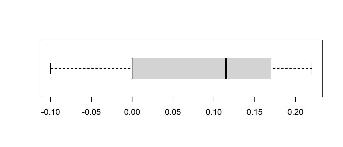
I will also double-check to make sure that the distribution of $D$ is “nearly normal” and doesn’t contain any outliers with an informal outlier check.

$$Min=-0.10, Q1=0, M=0.115, Q3=0.17, Max=0.22$$

$$IQR=0.17-0=0.17, Step=1.5 \times IQR=0.255$$

$$Q1-Step=0-0.255=-0.255, Q3+Step=0.17+0.255=0.425$$ There are no outliers. I will proceed with the $t$-test. What are called nonparametric tests are often used if there are outliers present that can’t be removed from the data; examples include the Wilcoxon Signed Rank Test and the Mann-Whitney Test (we will not study the formulas for these tests).

Step One: Write Hypotheses

$$H_O: \mu_D=0$$ $$H_A: \mu_D >0$$

Step Two: Choose Level of Significance

Let $\alpha=0.05$

Step Three: Choose Test & Check Assumptions I am satsified that we have a sample that is random, paired, with the difference satisfying the “nearly normal” condition, so I will use the paired samples t-test.

Step Four: Calculate the Test Statistic

$$t=\frac{\bar{D}-\mu_0}{s_D/\sqrt{n}}$$ $$t = \frac{0.09 - 0}{0.1086/\sqrt{10}}$$

$$t = \frac{0.09}{0.0343}$$

$$t=2.620$$

$$df=n-1=9$$

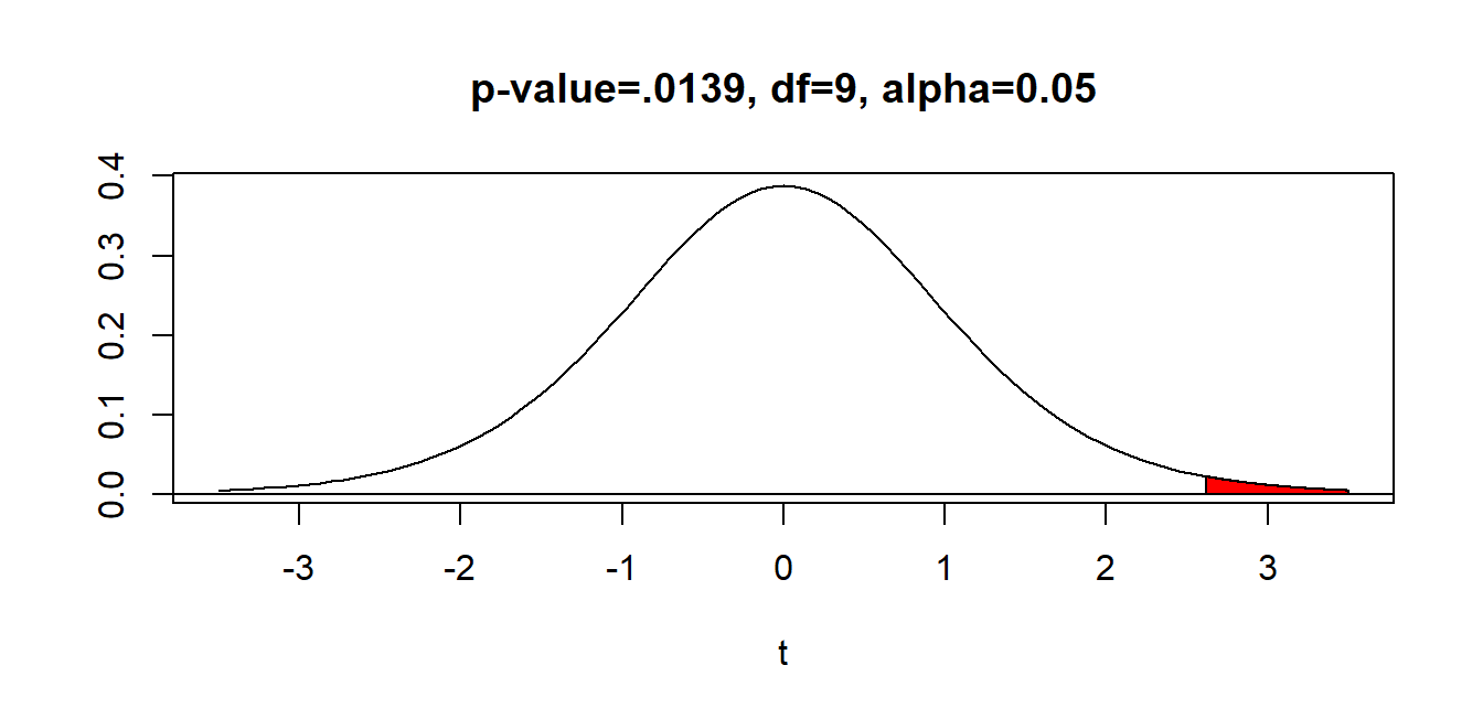
Step Five: Make a Statistical Decision (via the $p$-value)

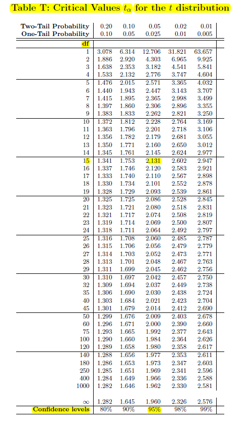
The $p$-value is $P(t>2.62)$. With $df=9$, notice our test statistic is between the critical values $t^*=2.262$ and $t^*=2.821$, which correspond to one-tail probabilities of $0.025$ and $0.01$, respectively. This means that $$0.01 < p-value < 0.025$$

Below is a picture showing the $p$-value, which can be computed with software to be $p=0.0139$, which as promised is more than $\alpha=0.01$ and less than $\alpha=0.025$.

Since we are using $\alpha=0.05$ and $p < \alpha$, we REJECT the null hypothesis.

Step Six: Conclusion

The mean difference in reaction time decrease significantly after the subject drank alcohol.

Below is what statistical output from the software package R would look like for this problem. I also included output for the Wilcoxon Signed Rank test (even though we will not cover the formula for this test). The software includes a one-sided confidence interval that I’ll ignore.

## 
##  Paired t-test
## 
## data:  Before and After
## t = -2.62, df = 9, p-value = 0.01391
## alternative hypothesis: true mean difference is less than 0
## 95 percent confidence interval:
##        -Inf -0.0270305
## sample estimates:
## mean difference 
##           -0.09

## 
##  Wilcoxon signed rank test with continuity correction
## 
## data:  Before and After
## V = 4, p-value = 0.01648
## alternative hypothesis: true location shift is less than 0

24.3 Independent Samples $t$-test

Here, we will cover how to test a hypothesis involving independent samples (also called the two-sample $t$-test). This is when we take measurements on subjects from two groups that are independnet of each other, to see if some sort of significant change has occurred.

Difference of Two Independent Means

Often we want to test the difference of means between two independent groups. For example, we want to compare the mean age of subjects assigned to the treatment group (call it $\mu_1$) and the mean age of subjects assigned to the control group (call it $\mu_2$). If we assume equal variances, the test statistic is:

$$t=\frac{\bar{x_1}-\bar{x_2}}{\sqrt{s_p^2(\frac{1}{n_1}+\frac{1}{n_2})}}$$

where $s_p^2$, the pooled variance is:

$$s_p^2=\frac{(n_1-1)s_1^2+(n_2-1)s_2^2}{n_1+n_2-2}$$

and the degrees of freedom are $df=n_1+n_2-2$

We have a sample of $n_1=16$ from the treatment group and $n_2=14$ people from the control group. The summary statistics are: $\bar{x_1}=55.7$ years, $s_1=3.2$, $\bar{x_2}=53.2$, $s_2=2.8$

We are testing for a significant difference (i.e. no direction), as we are interested in differences in either direction (the treatment group might be significantly older or younger).

Step One: Write Hypotheses

$$H_0: \mu_1=\mu_2$$ $$H_a: \mu_1 \neq \mu_2$$

Step Two: Choose Level of Significance

Let $\alpha=0.05$.

Step Three: Choose Test/Check Assumptions

I will choose the two-sample $t$-test. Assumptions include that the samples are independent, random, and normally distributed with equal variances. For this example, we will assume these are met without any further checks. The Wilcoxon Rank Sum (or Mann-Whitney) test is a nonparametric alternative if this nearly normal condition is violated.

Step Four: Compute the Test Statistic

$$s_p^2=\frac{(16-1)(3.2^2)+(14-1)(2.8^2)}{16+14-2}=\frac{255.52}{28}=9.1257$$ $$t=\frac{\bar{x_1}-\bar{x_2}}{\sqrt{s_p^2(\frac{1}{n_1}+\frac{1}{n_2})}}=\frac{55.7-53.2}{\sqrt{9.1257(\frac{1}{16}+\frac{1}{14})}}=\frac{2.5}{\sqrt{1.2222}}$$ $$t=2.261$$ $$df=n_1+n_2-2=16+14-2=28$$

Step 5: Find p-value, Make Decision

In our problem, we have the two-sided alternative hypothesis $H_a: \mu_1 \neq \mu_2$, a test statistic $t=2.261$, and $df=28$.

We refer to the row for $df=28$. Notice our test statistic $t=2.261$ falls between the critical values $t^*=2.048$ and $t^*=2.467$.

Because we have a two-sided test, our $p$-value is $.02<\text{p-value}<.05$.

Reject $H_0$ at $\alpha=.05$. We would have failed to reject $H_0$ if we had used $\alpha=0.01$.

TTable

Step Six: Conclusion

Since we rejected the null hypothesis, a proper conclusion would be:

The mean age of people in the treatment group is than the mean height of people in the control group.

Notice that the effect is said to be significantly different and NOT significantly greater. This is because we chose a two-sided alternative hypothesis rather than a one-sided hypothesis. This decision should be made a priori (before collecting data) and NOT changed just to get a ‘desired’ result.

24.4 Unequal Variances

The assumption of equal variances is sometimes not met, and an alternative version of the $t$-test exists when we assume unequal variances. This test is often called Welch’s $t'$-test.

$$t'=\frac{\bar{x_1}-\bar{x_2}}{\sqrt{\frac{s^2_1}{n_1}+\frac{s^2_2}{n_2}}}$$

Notice we do not need to compute $s_p^2$, pooled variance. However, the degrees of freedom are no longer equal to $n_1+n_2-2$. Instead, $df$ is either computed by an ugly formula (details hidden), approximated with an easier formula, or approximated even further by treating it as a $z$-test (for large samples).

Let’s look at another example, this time assuming unequal variances.

Example: Suppose I am comparing final exam scores for two different sections of the same course, with one class having taken their final exams on Monday morning and the other on Friday afternoon. We wish to see if there is a significant difference in scores.

Step One: Write Hypotheses

$$H_0: \mu_F=\mu_M$$ $$H_A: \mu_F \neq \mu_M$$

Step Two: Choose Level of Significance

Let $\alpha=0.05$.

Step Three: Choose Test/Check Assumptions

I will choose the two-sample $t$-test. Assumptions include that the samples are independent, random, and normally distributed with unequal variances. Notice there is an outlier in the Friday class, but it is a real score and I will not change or drop the score.

## ________________________________
##   1 | 2: represents 12, leaf unit: 1 
##     Monday$exam      Friday$exam
## ________________________________
##              |  2 |9            
##              |  3 |             
##             9|  4 |57           
##             3|  5 |             
##             3|  6 |23578        
##        875111|  7 |24           
##     987766311|  8 |027          
##             7|  9 |36           
##             0| 10 |             
## ________________________________
## n:         20      15       
## ________________________________

##   class min Q1 median Q3 max     mean       sd  n missing
## 1     F  29 62     68 82  96 68.66667 18.35626 15       0
## 2     M  49 71     81 87 100 78.65000 13.05565 20       0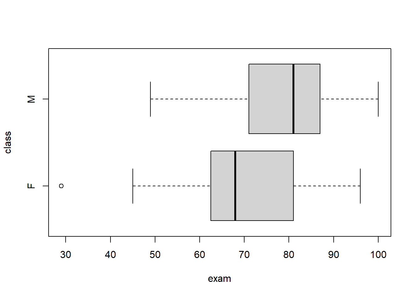

Step 4: Compute the test statistic

$$t'=\frac{\bar{x_1}-\bar{x_2}}{\sqrt{\frac{s^2_1}{n_1}+\frac{s^2_2}{n_2}}}$$ $$t'=\frac{68.66667-78.65}{\sqrt{\frac{18.35626^2}{15}+\frac{13.05565^2}{20}}}$$ $$t'=-1.793$$ Instead of using the complicated formula for degrees of freedom, I will use an approximation that will underestimate the df and thus provide a statistically conservative test that keeps $\alpha$ below the stated level of 0.05.

$$df \approx min(n_1-1,n_2-1) \approx min(14,19) \approx 14$$

Step 5: Find p-value, Make Decision

In our problem, we have the two-sided alternative hypothesis $H_a: \mu_1 \neq \mu_2$, a test statistic $t`=-1.793$, and $df \approx 14$.

We refer to the row for $df=14$. Notice the absolute value of our test statistic $|t'|=1.793$ falls between the critical values $t^*=1.761$ and $t^*=2.145$.

TTable

Because we have a two-sided test, our $p$-value is $.05<\text{p-value}<.10$.

Fail to reject $H_0$ at $\alpha=.05$. (What would it have been if I had made a one-sided hypothesis that scores were lower on Friday?)

Step 6: Make Conclusion The means of the final exam scores are not statistically different between Monday and Friday.

Here’s what the results look like when I used software. Notice the exact $df$ and $p$-value is computed by software so that an approximation for $df$ and a table are not needed. This result is more accurate. The software also computes a 95% confidence interval for the difference in the two means.

If you decided to NOT use a $t$-test based on the outlier, I’ve also included results from the Mann-Whitney test (called the Wilcoxon Rank Sum Test by my software), a non-parametric alternative (we will not cover its formula).

## 
##  Welch Two Sample t-test
## 
## data:  exam by class
## t = -1.7935, df = 24.084, p-value = 0.08547
## alternative hypothesis: true difference in means between group F and group M is not equal to 0
## 95 percent confidence interval:
##  -21.469922   1.503255
## sample estimates:
## mean in group F mean in group M 
##        68.66667        78.65000

## 
##  Wilcoxon rank sum test with continuity correction
## 
## data:  exam by class
## W = 96.5, p-value = 0.07706
## alternative hypothesis: true location shift is not equal to 0