Chapter 25 Meta-analysis
25.1 Defintion
The term meta-analysis refers too statistical techniques that are used to combine the results of several statistical studies together. This is done in an effort to objectively quantify the magnitude of effects (usually expressed as a correlation, a standardized mean difference, or a relative risk/odds ratio statistic) across several studies.
A less sophisticated way of doing this is vote-counting, which is merely obtaining a number of studies and counting how many of the studies are statistically significant, ignoring important aspects of the study including sample size, strength of effects measured, and the methodological quality of the research. For example, finding a significant effect (such as aspirin lowering one’s risk of heart disease) in one large study is probably more important than failing to find such an effect in several similar studies that were too small and suffered from a lack of statistical power.
There are also qualitative reviews of literature, which I certainly admit have their place.
25.2 What To Include
When one chooses to engage in a quantitative meta-analysis, several important decisions must be made by the meta-analyst.
Which studies to include (and possibly exclude) from the meta-analysis
How to compare and combine the results of the studies that are included.
In deciding which studies to include or exclude, the following are involved.
- Types of Studies–these can range from experiments conducted by famous scientists and publised in the most presitigious journals to studies by unknowns published in weaker journals to results that were never published in a peer-review journal, but are only available in a master’s thesis or doctoral disseration or conference proceeding or technical report (among others). These can be difficult to obtain and are sometimes referred to as the gray literature.
There is no completely objective way to decide whether a study is included or excluded from a study. Good judgement needs to be used in this decision. It is possible to assign weights to studies based on their perceived quality.
Timing of the Study–how far back in time one should go is going to be a decision that needs to be made on a case-by-case basis. At some point, it may no longer be appropriate to include studies from 20/30/40 years ago. There is no magic number of years that works in all cases.
Quality Control–As mentioned earlier, one can choose to leave out or assign lower weights to studies that are perceived to be of lower quality. This is a potential source of bias and some argue that all available studies should be used. It is also possible to set aside studies that are weaker and analyze them separately.
25.3 Combining Results
In deciding how to compare and combine results, one needs to think about:
Are the populations the same? The meta-analysis needs to determine in the included studies whether the populations are the same (or at least very similar) and the methodology is similar. Sometimes separate meta-analyses should be used for different sets of studies–an example we saw a few weeks ago looking at the relationship between the use of smokeless tobacco and stroke analyzed US studies and Swedish studies separately, largely because of differences between the smokeless tobacco products favored by American users versus Swedish users.
A technical decision is whether to use the fixed effects or random effects model for the meta-analysis. A fixed effects study assumes all studies include samples from similar populations, and that there is an overall fixed but unknown magnitude of the effect being tested, whether that effect is a standardized difference of means (null value of zero), a correlation (null value of zero), a relative risk or similar (null value of one), or some other statistic.
A random effects model assumes the population effect is different for each study, but consists of some overall effect plus some randon component specific to that study. The formulas are somewheat different depending on what is assumed.
A criticism of meta-analysis is that it is unlikely all studies for a particular hypothesis will be discovered and/or available to the meta-analysis. This is known as the file-drawer problem. One may not track down all articles, especially those published in obscure journals or in other languages. The gray literature (such as technical reports and student theses/dissertations) are often undiscovered. Publication bias can lead to studies that failed to find statistically significant results (i.e. \(p > 0.05\)) are more likely to be rejected by journal editors and remain unpublished and thus unknown to the meta-analyst. This publication bias also unfortunately can lead to p-hacking where researchers make an undue effort to obtain a \(p\)-value that is statistically significant. There is a movement to try to reduce p-hacking and publication bias based on whether \(p < 0.05\) or not with two-stage submission/acceptance, but this is not yet commonly used.
Also, if one chooses to include flawed or biased original studies in the meta-analysis, you may just be repeating mistakes made by others. Also, meta-analysis still only answers the question of statistical significance, not practical importance or clinical relevance.
A fail-safe number can be computed to estimate how many unknown non-significant results (i.e. papers stuck in the file drawer) would be needed in order to change the overall meta-analysis results from significant to non-significant. The idea is that if this fail-safe number is large, then we would have greater confidence in declaring that an overall significant result exists than if this fail-safe number is small.
25.4 The ‘Pygmalion’ Study example and the Forest Plot
Early example of meta-analysis: Do teacher expectations influence student achievement?
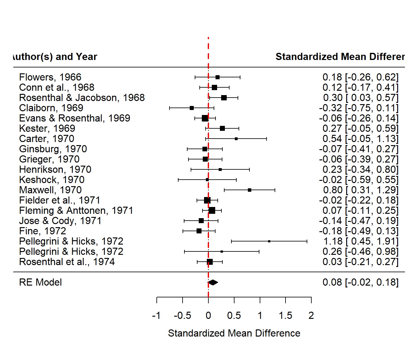
In the so-called ‘Pygmalion study’ (Rosenthal & Jacobson, 1968), “all of the predominantly poor children in the so-called Oak elementary school were administered a test pretentiously labeled the ‘Harvard Test of Inflected Acquisition.’ After explaining that this newly designed instrument had identified those children most likely to show dramatic intellectual growth during the coming year, the experimenters gave the names of these ‘bloomers’ to the teachers. In truth, the test was a traditional IQ test and the ‘bloomers’ were a randomly selected 20% of the student population. After retesting the children 8 months later, the experimenters reported that those predicted to bloom had in fact gained significantly more in total IQ (nearly 4 points) and reasoning IQ (7 points) than the control group children. Further, at the end of the study, the teachers rated the experimental children as intellectually more curious, happier, better adjusted, and less in need of approval than their control group peers” (Raudenbush, 1984).
In the following years, a series of studies were conducted attempting to replicate this rather controversial finding that teacher expectations play a major role in student learning. However, the great majority of those studies were unable to demonstrate a statistically significant difference between the two experimental groups in terms of IQ scores. Raudenbush (1984) conducted a meta-analysis based on 19 such studies to further examine the evidence for the existence of the ‘Pygmalion effect’. You may have heard it described as a ‘self-fulfilling prophecy’. The dataset includes the results from these studies.
The effect size measure used for the meta-analysis was the standardized mean difference (SMD), with positive values indicating that the supposed ‘bloomers’ had, on average, higher IQ scores than those in the control group. The null value for SMD is zero.
https://en.wikipedia.org/wiki/Pygmalion_effect
Rosenthal, R., & Jacobson, L. (1968). Pygmalion in the classroom. The Urban Review, 3(1), 16-20.
Raudenbush, S. W. (1984). Magnitude of teacher expectancy effects on pupil IQ as a function of the credibility of expectancy induction: A synthesis of findings from 18 experiments. Journal of Educational Psychology, 76, 85–97.
Raudenbush’s meta-analysis data, consisting of the Rosenthal-Jacobson study and 18 subsequent studies about the so-called Pygmalion effect is one of the sample data sets in a meta-analysis software package, which I used to recompute his results, shown in the forest plot.
##
## Fail-safe N Calculation Using the Rosenthal Approach
##
## Observed Significance Level: 0.0057
## Target Significance Level:   0.05
##
## Fail-safe N: 26
Notice while some individual studies (including the famous Rosenthal-Jacobson study from 1968) were statistically significant, indicated here with the confidence interval for the standardized mean difference, \((0.03, 0.57)\) lying completely above the null value of zero, that the overall meta-analysis results are not statisticall significant, \((-0.02, 0.18)\).
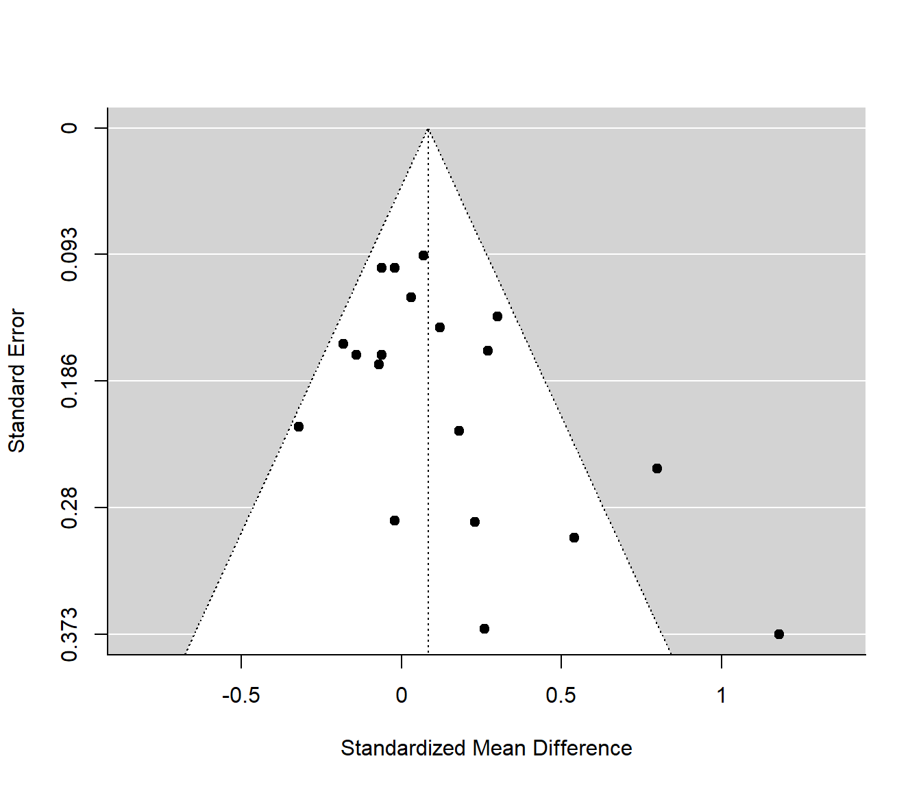
The funnel plot is a graph that is used to help detect study results that are outliers. The effect size and standard error are plotted for each study. Points that fall outside of the ‘funnel’ are often interpreted as indicating that publication bias exists. Reasons other than publication bias can lead to outliers, including but not limited to: poor methodological design, fraud, selective outcome reporting, sample size issues, poor statistical analysis, and random chance.
In the ‘Pygmalion case’, the Maxwell (1970) study, with \(SMD=0.8\) and the Pellegrini & Hicks (1972) study with \(SMD=1.18\), which happen to be the two largest standardized mean differences that were observed. There could be some publication bias present; I haven’t read any of these studies so I can’t comment on if issues with the quality of those studies exists. The fail safe-number is large: \(Fail-Safe \; N=26\).
25.5 Wine and Beer Consumption example
Meta-Analysis of Wine and Beer Consumption in Relation to Vascular Risk (relative risk)
Di Castelnuovo, A., Rotondo, S., Iacoviello, L., Donati, M. B., & De Gaetano, G. (2002). Meta-analysis of wine and beer consumption in relation to vascular risk. Circulation, 105(24), 2836-2844.

The confidence interval for the combined results in the included forest plot lies below 1, indicating a protective effect against vascular disease for small intake of wine. The article goes on to note a “J-shaped” relationship indicating that the risk eventually increases for large intake of wine.
25.6 Marital Quality example
Marital Quality and Personal Well-Being: A Meta-Analysis (correlations)
Proulx, C. M., Helms, H. M., & Buehler, C. (2007). Marital quality and personal well‐being: A meta‐analysis. Journal of Marriage and Family, 69(3), 576-593.
(no forest plot included in the article, unfortunately)
25.7 Poll Aggregators
Poll Aggregators (proportions/margins of error)
Nate Silver, might discuss briefly if time
https://fivethirtyeight.com/features/the-polls-are-all-right/
https://projects.fivethirtyeight.com/polls/kentucky/
