Chapter 23 Hypothesis Tests About One Mean

Here, we will cover how to construct boh a confidence interval and a hypothesis test when the parameter in question is the mean $\mu$ of a single sample, rather than a proportion. You’ll see that these tests will be similar to those covered for a proportion.

When the samples are large (generally considered to be when $n>30$), we can find an approximate test by using $z^*$ rather than $t^*$. As a statistician, I’d be using computer software and would use the slightly more accurate $t^*$.

TTable

23.1 Confidence Interval Based On the $t$ distribution (Review)

If $n=16$ (so $df=15$), $\bar{x}=192.4$ and $s=26.5$, then the 95% confidence interval for $\mu$ is: $$\bar{x} \pm t^* \frac{s}{\sqrt{n}}$$

$$192.4 \pm 2.131 \times \frac{26.5}{\sqrt{16}}$$

$$192.4 \pm 14.12$$

One could compute an approximate 95% confidence interval by using $t^* \approx 2$.

23.2 The $z$-test for a Single Mean

If the data were normally distributed and $\sigma$ was known, we could use the test statistic

$$z=\frac{\bar{x}-\mu_O}{\sigma/\sqrt{n}}$$

I’ll do an example loosely based on the Youtube video that considered the difference between statstical signficance and practical significance.

Researchers want to test a medication that is claimed to raise your intelligence, as measured by the IQ test, to a genius level (defined as 175+ in the video, which is 5 standard deviations above average, where organizations like Mensa use 3 standard deviations).

Suppose in the population, the average IQ score is $\mu=100$ and we assume $\sigma=15$. A sample of $n=40$ individuals is taken and we are testing to see if there was a significant change in the IQ scores.

Step One: Write Hypotheses

$$H_0: \mu=100$$ $$H_A: \mu \neq 100$$

Step Two: Choose Level of Significance

Let $\alpha=0.01$. (I’m using the second most common significance level for this problem, where it will be more difficult to reject the null and we will make fewer Type I errors, at the price of more Type II errors)

Step Three: Choose Test & Check Assumptions We will follow the textbook’s lead and use a $z$-test based on having a large sample that is assumed to be both random and normally distributed, with $\sigma$ known.

Step Four: Calculate the Test Statistic

Suppose that in our sample of $n=40$, we obtain $\bar{x}=110$.

$$z=\frac{\bar{x}-\mu_0}{\sigma/\sqrt{n}}$$ $$z = \frac{110 - 100}{15/\sqrt{40}}$$

$$z = \frac{10}{2.3717}$$

$$z=4.22$$ In WebAssign, they would call the numerator (10) the difference or the effect, the denominator (2.317) the standard error, and the 4.22 the standardized score or test statistic.

Step Five: Make a Statistical Decision (via the $p$-value)

Since the probability of $P(Z>4.22)$ is too small to be on the normal curve table, our $p$-value is very close to zero, I will say $p < .0001$. This is less than $\alpha=0.01$ and I will reject the null hypothesis.

Step Six: Conclusion

The mean IQ score is significantly different from 100. Note that this significance is in the statistical sense of the word significant. If the company was claiming your IQ would be raised to a genius level, this difference is certainly not that large, so this test may very well lack practical significance or clinical importance.

23.3 The $t$-test for a Single Mean

Since $\sigma$ will usually be unknown, let’s look at the test statistic.

$$t=\frac{\bar{x}-\mu_O}{s/\sqrt{n}}$$

This statistic will follow a $t$-distribution with $df=n-1$ when the null is true, and we will determine the decision rule and the $p$-value based on that $t$-distribution.

Example: The One-Sample $t$-test

Suppose we have a sample of $n=16$ seven-year-old boys from Kentucky. We have a hypothesis that these boys will be heavier than the national average of $\mu=52$ pounds. We will not assume that we have ‘magical’ knowledge about the value of $\sigma$.

Step One: Write Hypotheses

$$H_0: \mu=52$$ $$H_a: \mu > 52$$

Step Two: Choose Level of Significance

Let $\alpha=0.05$.

Step Three: Choose Test & Check Assumptions

Suppose the $n=16$ data values are: $$48 \quad 48 \quad 48 \quad 60 \quad 48 \quad 45 \quad 57 \quad 46$$ $$95 \quad 53 \quad 53 \quad 64 \quad 57 \quad 53 \quad 60 \quad 55$$

One boy seems to be an outlier. Maybe he is obese or very tall for his age. This data point might cause the distribution to be skewed and affect our ability to use the $t$-test!

Checking for Normality

One of the mathematical assumptions of the $t$-test is that the data is normally distributed. If we have a large sample, $n>30$, the Central Limit Theorem states that the sampling distribution of $\bar{x}$ will be approx. normal. We do not have a large sample.

The normal probability plot, or QQ-plot, is a graphical test for normality and can be made with software.

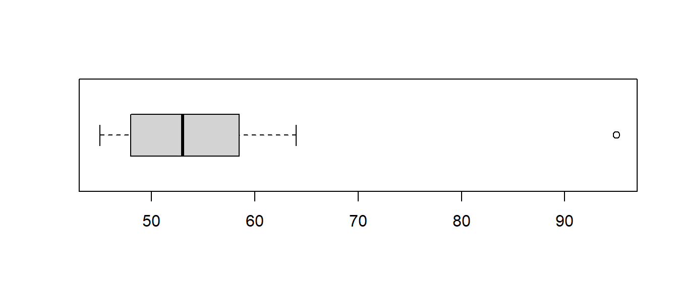
In practice, we can `bend the rules’ a bit and use the $t$-test as long as the data is close to symmetric and not heavily skewed with outliers. A boxplot can be used to check for this, which is easier to interpret. The heavy boy (boy #9) shows up as an outlier, which we do not want to see if we are planning on using a $t$-test with a small data set.

What to do about outliers?

Most statisticians do not consider it appropriate to delete an outlier unless there is both a statistical and a non-statistical reason for that deletion. Outliers can occur for several reasons: there might have been a data entry error (maybe that 95 was really 59), that observation might not belong to the population (maybe that boy was actually 11 years old), or it might be a true observation (that boy is obese and/or very tall for his age).

For our example, it was a data entry error. The boy was actually 59 pounds. The QQ plot and boxplot are fine when the point is corrected.

$$48 \quad 48 \quad 48 \quad 60 \quad 48 \quad 45 \quad 57 \quad 46$$ $$59 \quad 53 \quad 53 \quad 64 \quad 57 \quad 53 \quad 60 \quad 55$$

Back to our One-Sample $t$-test

In order to do Step Four and compute the test statistic, we need the sample mean and standard deviation of the weights. With the corrected value of 59, we get $\bar{x}=53.375$, $s=5.784$, $n=16$.

Step Four: Calculate the Test Statistic

$$t=\frac{\bar{x}-\mu_0}{s/\sqrt{n}}$$

$$t=\frac{53.375-52}{5.784/\sqrt{16}}=\frac{1.375}{1.446}=0.951$$

$$df=n-1=16-1=15$$

Step Five: Make a Statistical Decision (via the Decision Rule)

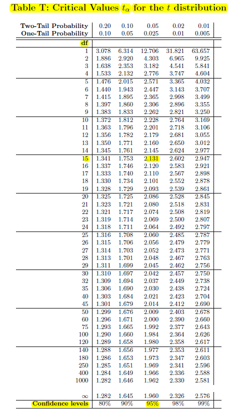
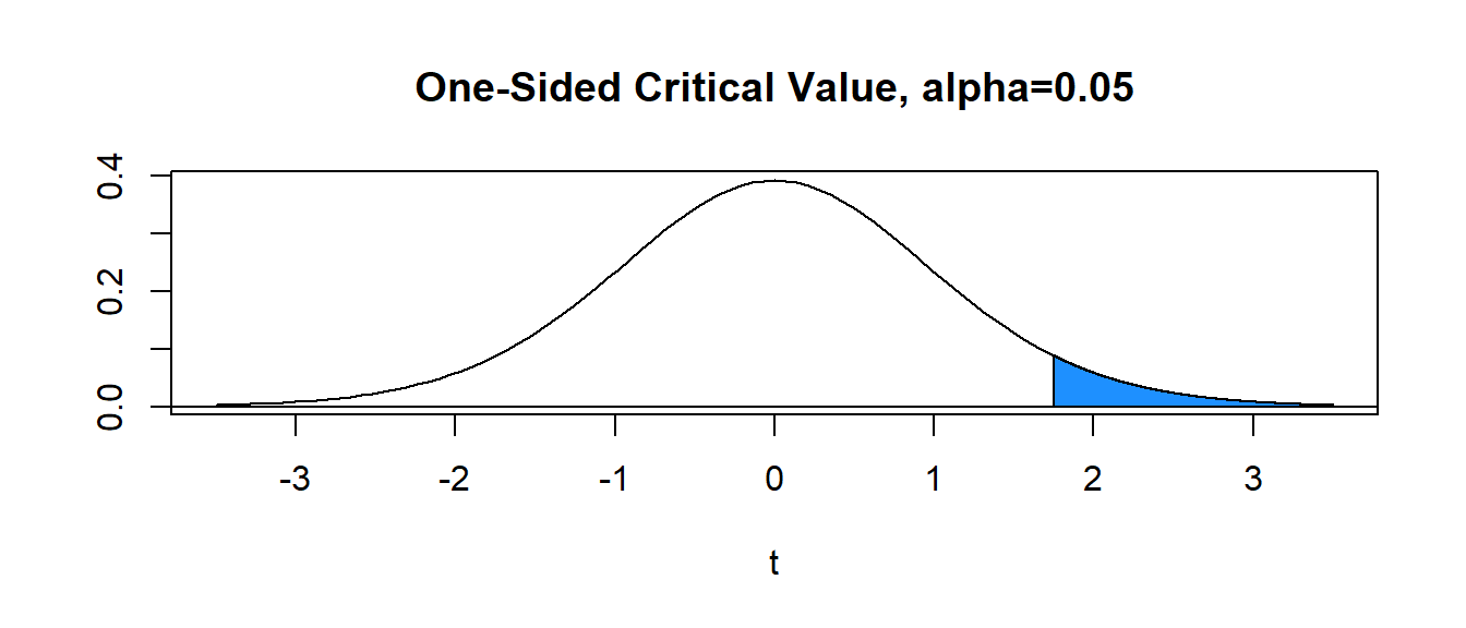
With $\alpha=0.05$ (area in blue) and $df=15$, the critical value is $t^*= 1.753$. Hence, the decision rule is to reject $H_0$ when the value of the computed test statistic $t$ exceeds critical value $t^*$, or reject $H_0$ if $t>t^*$. In our problem, $t=0.951 \not > 1.753=t^*$ and we FAIL TO REJECT the null.

Step Five: Make a Statistical Decision (via the $p$-value)

Computation of the $p$-value will be more difficult for us with the $t$-test than the $z$-test. The reason is that the $t$-table that is generally provided in statistical textbooks is much less extensive than the standard normal table. For us to be able to compute the exact $p$-value for a $t$-test, we need to:

• Have a two page $t$-table similar to the normal table for every possible value of $df$; that is, every row of the $t$-table would become two pages of probabilities. We do not have access to such tables. We can approximate the $p$-value with our one-page $t$-table.

• Evaluate the integral $P(t>0.951)=\int_{0.951}^{\infty} f(x) dx$, where $f(x)$ is the probability density function for the $t$-distribution with $n-1$ df. If you aren’t a math major, this may sound scary and awful! If you are a math major, you know this is scary and awful! So we won’t do it!

• Use techonology to get the $p$-value; that is, let the calculator or computer do the difficult math needed to compute the $p$-value.

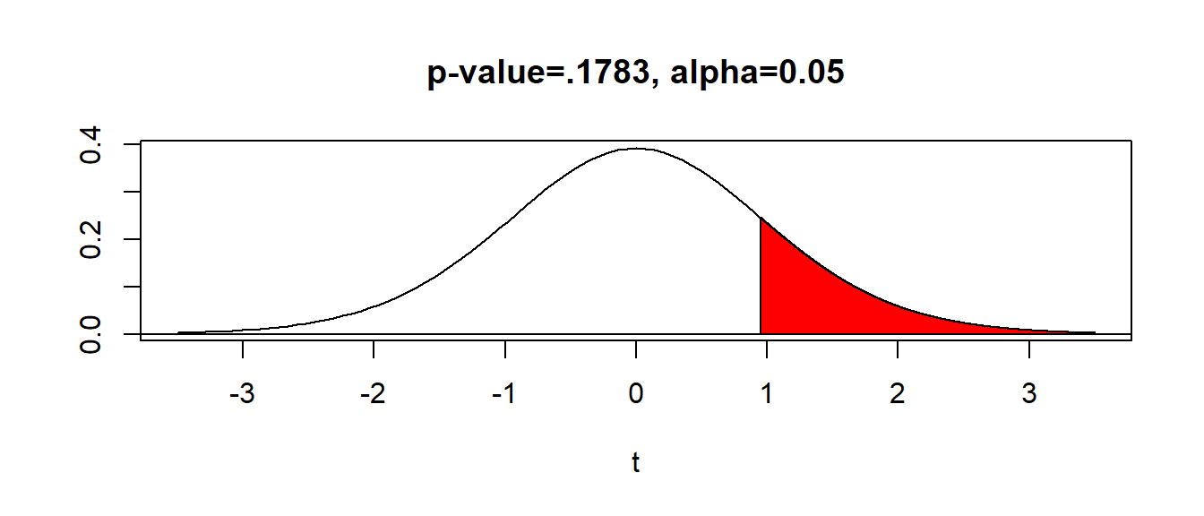
In our problem, we have the one-sided alternative hypothesis $H_a: \mu > 52$, a test statistic $t=0.951$, and $df=15$.

Below shows a $t$-table with the pertinent values highlighted. We refer to the row for $df=15$. Notice our test statistic $t=0.951$ falls below the critical values $t^*=1.341$.

The area above $t^*=1.341$ is .10. Hence, our $p$-value is greater than .10, or $\text{p-value}>.10$. If we had $H_a: \mu \neq 52$, then it would be $\text{p-value}>.20$.

TTable

The $p$-value can be obtained with technology. With a TI calculator (which I am not assuming you have), use tcdf(0.951,999999999,15) to get $p=0.1783$.

Step Six: Conclusion

Since we failed to reject the null hypothesis, a proper conclusion would be:

The mean weight of seven-year-old boys in Kentucky is NOT significantly greater than the national average of 52 pounds.