Chapter 8 Analysis of binary outcomes

Binary outcomes are ubiquitous in medical research and the comparison of binary outcomes in RCTs is very common. This chapter discusses various statistical quantities that can be calculated for comparing binary outcomes. We discuss statistical tests, suitable effect measures and methods to adjust for possible baseline variables.

8.1 Comparison of two proportions

Throughout this section, we will work with the following example.

Example 8.1 The APSAC Study is an RCT to compare a new thrombolytikum (APSAC) with the standard treatment (Heparin) in patients with acute cardiac infarction (Meinertz, Kasper, and Just 1988). The outcome is mortality within 28 days of hospital stay. Table 8.1 summarizes the results of this study, including 95% Wilson CIs for the proportion of patients who died in the respective treatment groups.

Table 8.1: Table 8.2: Results of the APSAC Study.
Therapy	Dead	Alive	Total	Percent Dead	Standard Error	95% Wilson-CI
APSAC	9	153	162	5.6%	1.8%	0.04 to 0.07
Heparin	19	132	151	12.6%	2.7%	0.1 to 0.2
Total	28	285	313

A visual comparison for the two separate CIs in Figure 8.1 shows that they overlap. However, overlapping CIs are not necessarily an indication for a non-significant treatment effect. Instead, we should rather look at CIs for combined effect measures such as the ones defined in Definition 8.1.

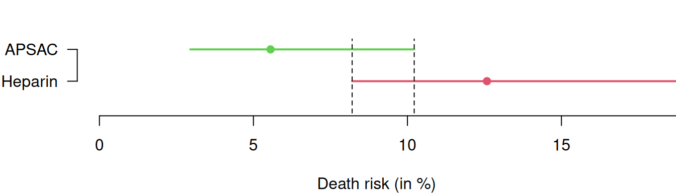
$95\% Wilson confidence intervals for the death risks in the APSAC Study.$

Figure 8.1: 95% Wilson confidence intervals for the death risks in the APSAC Study.

8.1.1 Statistical tests

Commonly used tests to compare two proportions are the and Fisher’s “exact” test, explained in Appendix B. The null hypothesis in these tests is that there is no difference between groups. Both methods give a $P$ -value, but no effect measure. There is a second version of the $\chi^2$ -test with continuity correction. There are at least three different versions to calculate the two-sided $P$ -value for Fisher’s exact’’ test (see the package for details). Fisher’s exact test should be used for small samples.

Example 8.2 R code for statistical tests comparing two proportions in the APSAC Study:

## observed number of cases
print(APSAC.table)

##         dead alive
## APSAC      9   153
## Heparin   19   132

## expected number of cases
print(chisq.test(APSAC.table)$expected)

##             dead   alive
## APSAC   14.49201 147.508
## Heparin 13.50799 137.492

# chi-squared test
chisq.test(APSAC.table)

## 
##  Pearson's Chi-squared test with Yates' continuity
##  correction
## 
## data:  APSAC.table
## X-squared = 3.9146, df = 1, p-value = 0.04787

chisq.test(APSAC.table, correct=FALSE)

## 
##  Pearson's Chi-squared test
## 
## data:  APSAC.table
## X-squared = 4.7381, df = 1, p-value = 0.0295

# Fisher's test
fisher.test(APSAC.table)

## 
##  Fisher's Exact Test for Count Data
## 
## data:  APSAC.table
## p-value = 0.04588
## alternative hypothesis: true odds ratio is not equal to 1
## 95 percent confidence interval:
##  0.1576402 0.9892510
## sample estimates:
## odds ratio 
##   0.409812

Note that the function fisher.test also provides an odds ratio (with 95% CI) as effect measure. The output from the $\chi^2$ -test can also be used to compute an estimate of the relative risk based on the observed to expected death ratios:

mytest <- chisq.test(APSAC.table)
o <- mytest$observed[,"dead"]
e <- mytest$expected[,"dead"]
print(ratio <- (o/e))

##     APSAC   Heparin 
## 0.6210317 1.4065752

## relative risk
print(RR <- ratio[1]/ratio[2])

##     APSAC 
## 0.4415205

8.1.2 Effect measures and confidence intervals

Let $\pi_0$ and $\pi_1$ be the true’’ risks of death in the Control and APSAC group, respectively with $\pi_0 \geq \pi_1$ . The following quantities are used to compare $\pi_0$ and $\pi_1$ :

Definition 8.1 The absolute risk reduction is defined as $\mbox{ARR}= \pi_0-\pi_1.$

The number needed to treat is defined as $\mbox{NNT}= 1 / \mbox{ARR}.$

The relative risk is defined as $\mbox{RR}= {\pi_1}/{\pi_0}.$

The relative risk reduction is defined as $\mbox{RRR}= \frac{\mbox{ARR}}{\pi_0} = 1 - \mbox{RR}.$

The odds ratio is defined as $\mbox{OR}= \frac{\pi_1/(1-\pi_1)}{\pi_0/(1-\pi_0)}.$

No difference between groups (i.e. $\pi_0 = \pi_1$ ) corresponds to $\mbox{ARR}=\mbox{RRR}=0$ and $\mbox{RR}=\mbox{OR}=1$ . We now discuss each of these effect measures together with their CIs for the example of the APSAC Study.

8.1.2.1 Absolute Risk Reduction

The ARR is also called risk difference ( $\mbox{RD}$ ) or probability difference. The estimated ARR

$\widehat{\mbox{ARR}} \ = \ 12.6\%-5.6\%=7\%$

with standard error

$\mbox{se}(\widehat{\mbox{ARR}}) = \sqrt{\frac{\hat \pi_0 (1-\hat \pi_0)}{n_0}+\frac{\hat \pi_1 (1-\hat \pi_1)}{n_1}}= 3.2\%$

Here we obtain $\mbox{se}(\widehat{\mbox{RD}}) = 3.2\%$ . can be used to calculate a Wald CI for the ARR. An improved Wilson CI for the ARR can be calculated using the square-and-add’’ approach (Robert G. Newcombe 1998b,Newcombe), see Appendix A.2.3 for details. (Newcombe, 1998).

Example 8.3 The following R code provides both Wald and Wilson CIs for the ARR in the APSAC Study. They are visually compared in Figure 8.2. There are no large differences between the two types of confidence intervals, only the upper limit of the Wilson is slightly larger than the corresponding Wald upper limit.

library(biostatUZH)
x <- c(19, 9)
n <- c(151, 162)
print(confIntRiskDiff(x, n))

## $rd
##            [,1]
## [1,] 0.07027226
## 
## $CIs
##     type       lower     upper
## 1   Wald 0.006691788 0.1338527
## 2 Wilson 0.006303897 0.1378381

The lower plot in Figure 8.2 illustrates the distinct advantage of the Wilson CI that it avoids overshoot with artificial data. Indeed, the upper limit of the Wald confidence interval for the risk difference is larger than 1 whereas this is not the case for the Wilson interval.

x.art <- c(11,1)
n.art <- c(12,12)
print(confIntRiskDiff(x.art, n.art))

## $rd
##           [,1]
## [1,] 0.8333333
## 
## $CIs
##     type     lower    upper
## 1   Wald 0.6121830 1.054484
## 2 Wilson 0.4507227 0.930162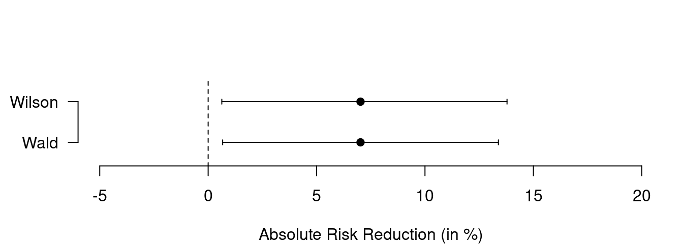

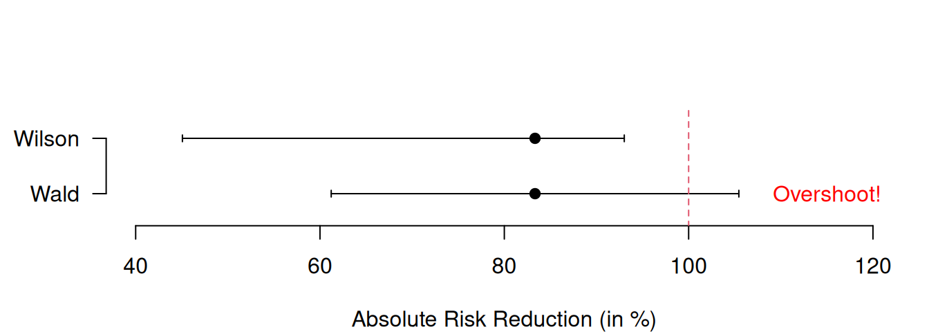
Figure 8.2: Wald and Wilson CIs for the ARR in the APSAC Study (upper plot) and in an example with artifical data illustrating overshoot (lower plot).

8.1.2.2 Number Needed to Treat

Suppose we have $n$ patients in each treatment group. The expected number of deaths in the control and intervention group are: $\begin{eqnarray*} N_0 & = & n \, \pi_0, \\ N_1 & = & n \, \pi_1. \end{eqnarray*}$ The difference is therefore $N_0-N_1 = n \, (\pi_0-\pi_1)$ . Suppose we want the difference $N_0 - N_1$ to be one patient. The required sample size $n$ to achieve this is $n = 1/(\pi_0-\pi_1) = 1/\mbox{ARR}.$ This is the number needed to treat, the required number of patients to be treated with the intervention rather than control to avoid one death. Depending on the direction of the effect, the NNT is also called number needed to benefit or number needed to harm.

The interpretation of the estimated $\mbox{NNT}$ % $\quad \widehat{\mbox{NNT}} \ = \ 1/\widehat{\mbox{ARR}} \ = \ 1 / 0.07 \ = \ 14.2$ % in the APSAC study is the following: To avoid one death, we need to treat $\widehat{\mbox{NNT}} = 14.2$ patients with APSAC rather than with Heparin. A CI for $\mbox{NNT}$ can be obtained by inverting the limits $\mbox{L}_{\mbox{\scriptsize ARR}}$ and $\mbox{U}_{\mbox{\scriptsize ARR}}$ of the CI for $\mbox{ARR}$ .

Example 8.4 The following R code shows this for the APSAC Study.

(ci.arr <- confIntRiskDiff(x, n)$CIs[2,])

##     type       lower     upper
## 2 Wilson 0.006303897 0.1378381

ci.ntt <- 1/ci.arr[c(3,2)]
colnames(ci.ntt) <- c("lower", "upper")
print(round(ci.ntt, 1))

##   lower upper
## 2   7.3 158.6

The CI for $\mbox{NNT}$ in the APSAC Study is: $1 / 0.138$ to $1 / 0.006$ = $7.3$ to $158.6$ .

Note that the CI for $\mbox{NNT}$ is only well-defined as long as the CI for $\mbox{ARR}$ does not contain 0. Otherwise, the confidence interval is actually a confidence region, comprising two different intervals depending on the direction of the treatment effect (Douglas G. Altman 1998). This problem can be circumvented by plotting the number needed to treat on the absolute risk reduction scale, as illustrated in the following example.

Example 8.5 Figure 8.3 shows a forest plot from Douglas G. Altman (1998) where an overall number needed to benefit is calculated from a meta-analysis of data from randomized trials comparing bypass surgery with coronary angioplasty in relation to angina in one year. For three studies (CABRI, RITA, EAST) the 95% confidence interval for NNT is a regular interval and includes only values that indicate a benefit of therapy. However, for two other entries (GABI and Other) the confidence region for NNT splits into two intervals. For example, for GABI the two intervals are 7.5 to infinity for benefit and 14.5 to infinity for harm. This indicates that this trial is inconclusive regarding the direction of the treatment effect with large uncertainty regarding the actual value of NNT.

Forest plot for NNT in a meta-analysis [@altman1998].

Figure 8.3: Forest plot for NNT in a meta-analysis (Douglas G. Altman 1998).

8.1.2.3 Relative Risk

The RR is also called risk ratio. The estimated death risks in both treatment groups are

$x_1/n_1=9/162=5.6\%$ for APSAC and
$x_0/n_0=19/151=12.6\%$ for Heparin.

The estimated RR is therefore

$\widehat{\mbox{RR}} = \frac{5.6\%}{12.6\%} = 0.44.$

The calculation of a CI for the RR is based on the RR as explained in Table 8.3. With the standard error of the log RR

$\mbox{se}(\color{red}{\log}(\widehat{\mbox{RR}})) = \sqrt{\frac{1}{x_1}-\frac{1}{n_1}+\frac{1}{x_0}-\frac{1}{n_0}}$

and the corresponding $\mbox{EF}_{.95} = \exp\left\{1.96 \cdot \mbox{se}(\color{red}{\log}(\widehat{\mbox{RR}}))\right\},$ we can directly calculate the limits of the CI for the RR as

$\begin{equation} \tag{8.1} \widehat{\mbox{RR}}/\mbox{EF}_{.95} \text{ and } \widehat{\mbox{RR}} \cdot \mbox{EF}_{.95}. \end{equation}$

Example 8.6 This calculation is implemented in the function from package .

x <- rev(x)
n <- rev(n)
(ci.rr <- confIntRiskRatio(x, n))

##      lower Risk Ratio      upper 
##  0.2061781  0.4415205  0.9454948

We can see that the data are compatible with a relative risk between 0.21 and 0.95.

Table 8.3: Calculation of a CI for the RR based on the log RR.
Quantity	Estimate	Standard Error	95%-confidence interval
RR	0.44		0.21 to 0.95
	↓ log ↓		↑ exp ↑
RR	-0.82	0.39	-1.58 to -0.06

The square-and-add method can also be applied to ratio measures such as the risk ratio R. G. Newcombe (2013) (Section 7.3.4), but this is rarely used in practice. One reason might be that the simple approach (8.1) based on error factors is - by construction - not prone to overshoot below zero.

8.1.2.4 Relative Risk Reduction

Either ARR or RR can be used to estimate $\mbox{RRR}$ : $\begin{eqnarray*} \widehat{\mbox{RRR}} & = & \frac{\widehat{\mbox{ARR}}}{\widehat{\pi}_0} \ = \ \frac{0.07}{0.126} \ = \ 56\% \mbox{ or} \\ \widehat{\mbox{RRR}} & = & 1-\widehat{\mbox{RR}} \ = \ 1 - 0.44 \ = \ 56\% \end{eqnarray*}$ A CI for $\mbox{RRR}$ can be obtained based on the limits $\mbox{L}_{\mbox{\scriptsize RR}}$ and $\mbox{U}_{\mbox{\scriptsize RR}}$ of the CI for $\mbox{RR}$ :

$\begin{eqnarray*} (1 - \mbox{U}_{\mbox{\scriptsize RR}}) \mbox{ to } (1 - \mbox{L}_{\mbox{\scriptsize RR}}) & = & (1 - 0.95) \mbox{ to } (1 - 0.21) \\ & = & 0.05 \mbox{ to } 0.79 \end{eqnarray*}$

So, the risk of death with APSAC has been reduced by 56% (95% CI: 5% to 79%) compared to Heparin.

8.1.2.5 Odds Ratio

Table 8.4: Table 8.5: $2\times 2$ table for the APSAC Study.
	Dead
	Yes	No	Total
APSAC	$a=9$	$b=153$	162
Heparin	$c=19$	$d=132$	151
			n=313

From Table 8.4, we can read that the estimated odds of death for APSAC are $a/b = 9/153$ ( $c/d=19/132$ for Heparin). The estimated OR is therefore $\widehat{\mbox{OR}} = \frac{a / b}{c / d} = \frac{9 / 153}{19 / 132} = \frac{9 \cdot 132}{153 \cdot 19} \ = 0.41.$ This means that the odds of death are under APSAC 59% lower than under Heparin treatment. The formulation $\widehat{\mbox{OR}}=(a\cdot d) / (b \cdot c)$ motivates the alternative name cross-product ratio.

Table 8.6: Table 8.7: Considering survival probability in the APSAC Study.
	Dead	Alive	Total	Percent Alive	Standard Error	95% CI
APSAC	9	153	162	94.4%	1.8%	98.0 to 90.9%
Heparin	19	132	151	87.4%	2.7%	92.7 to 82.1%

An advantage of the ORs is that they can be inverted for complementary events. If we consider the survival probability rather than the death risk as in Table 8.6, we can see that:

The odds ratio for death risk is $\mbox{OR}=0.41$ .
The odds ratio for survival then is

$\frac{(1-\pi_1)/\pi_1}{(1-\pi_0)/\pi_0} = \frac{\pi_0/(1-\pi_0)}{\pi_1/(1-\pi_1)} = 1/\mbox{OR}= 1/0.41 = 2.45.$

Such a relationship does not hold for relative risks: $1/\mbox{RR}= 1/0.44 = 2.25, \mbox{ but } 94.4\%/87.4\% = 1.08.$

A disadvantage of the ORs is their noncollapsibility (S. Senn 2021). Consider an example: Table 8.8 presents a contingency table stratified by strata while Table 8.10 present the collapsed contingeny table.

Table 8.8: Table 8.9: Stratified contingency table
	Stratum 1			Stratum 2
	Yes	No	Total	Yes	No	Total
Therapy A	10	20	30	15	25	40
Therapy B	30	40	70	35	45	80

Table 8.10: Table 8.11: Collapsed contingency table
	Yes	No	Total
Therapy A	10	20	30
Therapy B	30	40	70

The OR for Stratum 1 is $\mbox{OR} = \frac{10 \cdot 40}{20 \cdot 30} = 2.67$
The OR for Stratum 2 is $\mbox{OR} = \frac{15 \cdot 45}{25 \cdot 35} = 2.67$
The OR from the collapsed analysis is $\mbox{OR} = \frac{10 \cdot 40}{20 \cdot 30} = 2.53$
[ $\rightarrow$ ] The ORs are the same in both strata, but the OR collapsed over strata is different

As for $\mbox{RR}$ (see Table 8.3), we calculate the standard error of the OR on the log scale: $\mbox{se}(\color{red}{\log}(\widehat{\mbox{OR}})) = \sqrt{\frac{1}{a}+\frac{1}{b}+\frac{1}{c}+\frac{1}{d}}$

The CI can be directly calculated using the 95% error factor % $\mbox{EF}_{.95} = \exp\left\{1.96 \cdot \mbox{se}(\color{red}{\log}(\widehat{\mbox{OR}}))\right\}$ Note that CIs for odds ratios may differ even if group sample sizes remain the same:

x <- c(25, 25)
n <- c(50, 50)
(ci.or1 <- confIntOddsRatio(x, n))

##      lower Odds Ratio      upper 
##  0.4565826  1.0000000  2.1901841

x <- c(1, 1)
n <- c(50, 50)
(ci.or2 <- confIntOddsRatio(x, n))

##       lower  Odds Ratio       upper 
##  0.06081319  1.00000000 16.44380070

8.1.2.6 Odds Ratios and Relative Risks

There are the following relations between the OR and the RR:

If $\pi_0=\pi_1$ then $\mbox{OR}= \mbox{RR}= 1$
OR and RR always go in the same direction ( $<1$ or $>1$ )
If $<1$ , then $\mbox{OR}< \mbox{RR}$
If $>1$ , then $\mbox{OR}> \mbox{RR}$
Rare disease assumption: If disease risks $\pi_0$ and $\pi_1$ are small, then $\mbox{OR}\approx \mbox{RR}$

Example 8.7 The twoby2 function from the R package Epi computes the RR (relative risk), OR (in two versions) and ARR (probability difference). The second version of the odds ratio is the conditional Maximum Likelihood estimate under a hypergeometric likelihood function. There is no closed-form expression for this estimate, which may explain why it is rarely used, but it is compatible to the $p$ -value from Fisher’s exact test (denoted here as Exact P-value).

library(Epi)
twoby2(APSAC.table)

## 2 by 2 table analysis: 
## ------------------------------------------------------ 
## Outcome   : dead 
## Comparing : APSAC vs. Heparin 
## 
##         dead alive    P(dead) 95% conf. interval
## APSAC      9   153     0.0556    0.0292   0.1033
## Heparin   19   132     0.1258    0.0817   0.1889
## 
##                                     95% conf. interval
##              Relative Risk:  0.4415    0.2062   0.9455
##          Sample Odds Ratio:  0.4087    0.1788   0.9340
## Conditional MLE Odds Ratio:  0.4098    0.1576   0.9893
##     Probability difference: -0.0703   -0.1378  -0.0063
## 
##              Exact P-value: 0.0459 
##         Asymptotic P-value: 0.0338 
## ------------------------------------------------------

Compatible $p$ -values can be obtained for each of these effect estimates and the corresponding standard error. They will be similar, but not identical:

## transform normal test statistic z to two-sided p-value
z2p <- function(z) return(2*(1-pnorm(abs(z))))

z <- c(arr/se.arr, log(rr)/se.log.rr, log(or)/se.log.or)
names(z) <- c("risk difference", "log relative risk", "log odds ratio")
pvalues <- z2p(z)
formatPval(pvalues)

## [1] "0.03" "0.04" "0.03"

The one for OR is called in .

8.1.2.7 Absolute and relative effect measures

Let us consider an example of an RCT with $\begin{eqnarray*} \mbox{death risk} &= & \left\{ \begin{array}{rl} 0.3\% & \mbox{in the placebo group} \\ 0.1\% & \mbox{in the treatment group} \end{array} \right. \end{eqnarray*}$ Then we have $\mbox{ARR}=0.2\%= 0.002$ and $\mbox{NNT}=500$ , so there is a very small absolute effect of treatment. However, we have $\mbox{RR}=1/3$ and $\mbox{RRR}= 2/3 = 67\%$ , so there is a large relative effect of treatment. We cannot transform absolute to relative effect measures (and vice versa) without knowledge of the underlying risks.

8.2 Adjusting for baseline

For binary outcomes, adjusting for baseline variables is usually done using logistic regression and will produce adjusted odds ratios. Alternatively, the Mantel-Haenszel method (MH) can be used, which gives a weighted average of strata-specific odds ratios. The MH method can also be applied to strata-specific risk ratios. However, adjustment for continuous variables using MH is only possible after suitable categorization.

8.2.1 Logistic regression

Example 8.8 PUVA

The PUVA trial compares PUVA (drug followed by UVA exposure) versus TL-01 lamp therapy for treatment of psoriasis. The primary outcome is yes if the patient was clear of psoriasis at or before the end of the treatment, and no otherwise. The treatment allocation used RPBs stratified according to whether predominant plaque size was large or small. This ensures a balanced distribution in treatment arms (29:22 vs. 28:21).

print(puva)

##   plaqueSize treatment cleared total
## 1      Small     TL-01      23    29
## 3      Small      PUVA      25    28
## 2      Large     TL-01       9    22
## 4      Large      PUVA      16    21

Unadjusted analysis:

m1 <- glm(cbind(cleared, total-cleared) ~ treatment, 
          data=puva, family=binomial)
## tableRegression gives profile confidence intervals
knitr::kable(tableRegression(m1, latex = FALSE))

% latex table generated in R 4.4.1 by xtable 1.8-4 package % Fri Oct 4 10:19:11 2024

	Odds Ratio	95%-confidence interval	$p$ -value
treatmentTL-01	0.33	from 0.12 to 0.82	0.021

With standard formulae (p. 18):

(x <- rev(by(data=puva$cleared, INDICES=puva$treatment, FUN=sum)))

## puva$treatment
## TL-01  PUVA 
##    32    41

(n <- rev(by(data=puva$total, INDICES=puva$treatment, FUN=sum)))

## puva$treatment
## TL-01  PUVA 
##    51    49

round(confIntOddsRatio(x=as.numeric(x), n=as.numeric(n)), 2)

##      lower Odds Ratio      upper 
##       0.13       0.33       0.85

Strata-specific estimates:

m2Small <- glm(cbind(cleared, total-cleared) ~ treatment, 
          subset=(plaqueSize=="Small"), data=puva, family=binomial)
knitr::kable(tableRegression(m2Small, latex = FALSE))

% latex table generated in R 4.4.1 by xtable 1.8-4 package % Fri Oct 4 10:19:11 2024

	Odds Ratio	95%-confidence interval	$p$ -value
treatmentTL-01	0.46	from 0.09 to 1.96	0.31

m2Large <- glm(cbind(cleared, total-cleared) ~ treatment, 
          subset=(plaqueSize=="Large"), data=puva, family=binomial)
knitr::kable(tableRegression(m2Large, latex = FALSE))

% latex table generated in R 4.4.1 by xtable 1.8-4 package % Fri Oct 4 10:19:11 2024

	Odds Ratio	95%-confidence interval	$p$ -value
treatmentTL-01	0.22	from 0.05 to 0.77	0.023

Adjusted analysis with logistic regression:

m3 <- glm(cbind(cleared, total-cleared) ~ treatment + plaqueSize, 
          data=puva, family=binomial)
knitr::kable(tableRegression(m3, latex = FALSE))

% latex table generated in R 4.4.1 by xtable 1.8-4 package % Fri Oct 4 10:19:11 2024

	Odds Ratio	95%-confidence interval	$p$ -value
treatmentTL-01	0.30	from 0.10 to 0.78	0.017
plaqueSizeLarge	0.24	from 0.09 to 0.61	0.004

The adjusted treatment effect is $\widehat{\mbox{OR}} = 0.30$ with 95% CI from $0.10$ to $0.78$ . Logistic regression also quantifies the effect of the variable used for adjustment, here plaque size.

8.3 Additional references

Relevant references for this chapter are in particular Chapters 13 “The Analysis of Cross-Tabulations” and 15.10 “Logistic Regression” in M. Bland (2015) as well as Chapter 7.1–7.4 “Further Analysis: Binary Data” in J. N. S. Matthews (2006). The use of odds ratios is discussed in Sackett, Deeks, and Altman (1996) and Douglas G. Altman, Deeks, and Sackett (1998). Studies where the methods from this chapter are used in practice are for example Heal et al. (2009),fagerstroem and Vadillo-Ortega et al. (2011).

References

———. 1998. “Confidence intervals for the number needed to treat.” BMJ 317: 1309–12.

Altman, Douglas G, Jonathon J Deeks, and David L Sackett. 1998. “Odds Ratios Should Be Avoided When Events Are Common.” BMJ 317 (7168): 1318.

Bland, Martin. 2015. An Introduction to Medical Statistics. Fourth. Oxford University Press.

Heal, Clare F, Petra G Buettner, Robert Cruickshank, David Graham, Sheldon Browning, Jayne Pendergast, Herwig Drobetz, Robert Gluer, and Carl Lisec. 2009. “Does single application of topical chloramphenicol to high risk sutured wounds reduce incidence of wound infection after minor surgery? Prospective randomised placebo controlled double blind trial.” BMJ 338: 1–6.

Matthews, John N. S. 2006. Introduction to Randomized Controlled Clinical Trials. Second. Chapman & Hall/CRC.

Meinertz, Thomas, Martin Kasper Wolfgang Schumacher, and Hanjörg Just. 1988. “The German multicenter trial of anisoylated plasminogen streptokinase activator complex versus heparin for acute myocardial infarction.” Am J Card 62 (7): 347–51.

Newcombe, R. G. 2013. Confidence Intervals for Proportions and Related Measures of Effect Size. Boca Ration, FL: Chapman & Hall/CRC.

———. 1998b. “Interval estimation for the difference between independent proportions: Comparison of eleven methods.” Stat Med 17 (8): 873–90.

Sackett, David L, Jonathan J Deeks, and Douglas G Altman. 1996. “Down with Odds Ratios!” BMJ Evidence-Based Medicine 1 (6): 164–66.

———. 2021. Statistical Issues in Drug Development. Third. Ney York: Wiley.

Vadillo-Ortega, Felipe, Otilia Perichart-Perera, Salvador Espino, Marco Antonio Avila-Vergara, Isabel Ibarra, Roberto Ahued, Myrna Godines, Samuel Parry, George Macones, and Jerome F Strauss. 2011. “Effect of supplementation during pregnancy with L-arginine and antioxidant vitamins in medical food on pre-eclampsia in high risk population: randomised controlled trial.” BMJ 342.