6.4 PLSC Analysis

pls <- tepPLS(basic.taste,others, DESIGN = wk0$Product, make_design_nominal = FALSE, graphs = TRUE)

## [1] "DESIGN is not dummy-coded matrix. Creating default."

6.4.1 Scree Plot

Note that here we need to use the “perm4PLSC” function to perform the permutation inference test. This will help find the p.values associated with each eigenvalues that we can use to (1) augment our Scree Plot and (2) to perform eigen value tests. Also, note that there is no inference.battery function to find all inference results for PLSC yet. THis is why we will need to remember to set permType parameter to “byColumn” so that we can permute all cols of each data matrix independently. The default option type is “byMat” which permute by labels of observations. In order to extract the info needed for p.values of eigenvalues, we need to use “$pEigenvalues”.From the scree plot we see that the first 2 components are note-worthy to take a deeper look at compared to the other components.

# permuation tests byColumns
nIter <- 1000 #set the number of iterations to run the permutation test 

perm.bycol <- perm4PLSC(basic.taste, 
                        others, 
                        permType = 'byColumns', # the default type is byMat which permute by labels of observations
                                                # byColumns option permutes all cols of each data matrix independently
                        nIter = nIter)

scree      <- PlotScree(ev = pls$TExPosition.Data$eigs,
                        p.ev = perm.bycol$pEigenvalues,
                        title = "Explained Variance per Dimension + Permutation Tests",
                        plotKaiser = TRUE)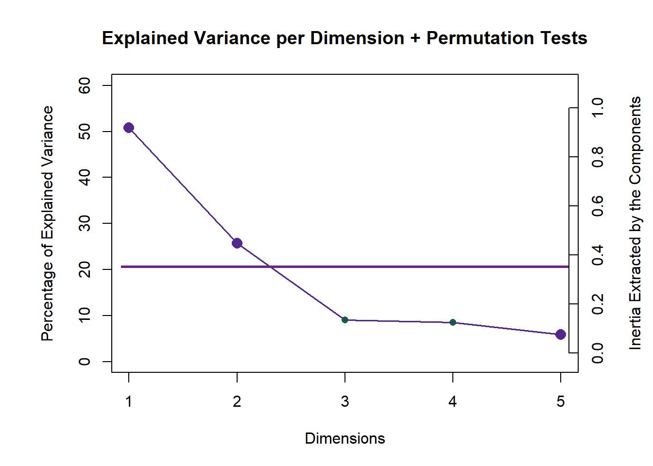

scree1     <- recordPlot()

6.4.2 Rows Factor Scores

6.4.2.1 Sample Code to find 1st latent variable of both tables - Sausage Type Perspective

# For the first plot, the first component of the latent variable of X is the x-axis, and the first component of the latent variable of Y is the y-axis
lv.1 <- cbind(pls$TExPosition.Data$lx[,1],pls$TExPosition.Data$ly[,1])

assign.type <- ifelse(wk0[,3] == 1, "Pavo", "Viena") #assign sausage type
rownames(lv.1) <- assign.type

# compute means
lv.1.mean <- getMeans(lv.1, wk0$Session)
row.names(lv.1.mean) <- c("Pavo", "Viena")

#Color by sausage type means
prod.color.type.mean <- dplyr::recode(rownames(lv.1.mean),
                       'Pavo' = 'green3',
                       'Viena' = 'orange',
                       )

# get bootstrap intervals of groups
lv.1.mean.boot <- Boot4Mean(lv.1, wk0$Session)

# Let's Plot it!
plot1.lv.1 <- createFactorMap(lv.1,
                         col.points = prod.color.type,
                         col.labels = prod.color.type,
                         alpha.points = 0.2
                         )

plot1.mean <- createFactorMap(lv.1.mean,
                              col.points = prod.color.type.mean,
                              col.labels = prod.color.type.mean,
                              cex = 4,
                              pch = 17,
                              alpha.points = 0.8)

plot1.meanCI <- MakeCIEllipses(lv.1.mean.boot$BootCube[,c(1:2),], # get the first two components
                              col = prod.color.type.mean
                              )

plot1 <- plot1.lv.1$zeMap_background + 
         plot1.lv.1$zeMap_dots + 
         plot1.mean$zeMap_dots + 
         plot1.mean$zeMap_text + 
         plot1.meanCI +
         ggtitle("Latent 1: Observations Factor Scores (by Sausage Type)") +
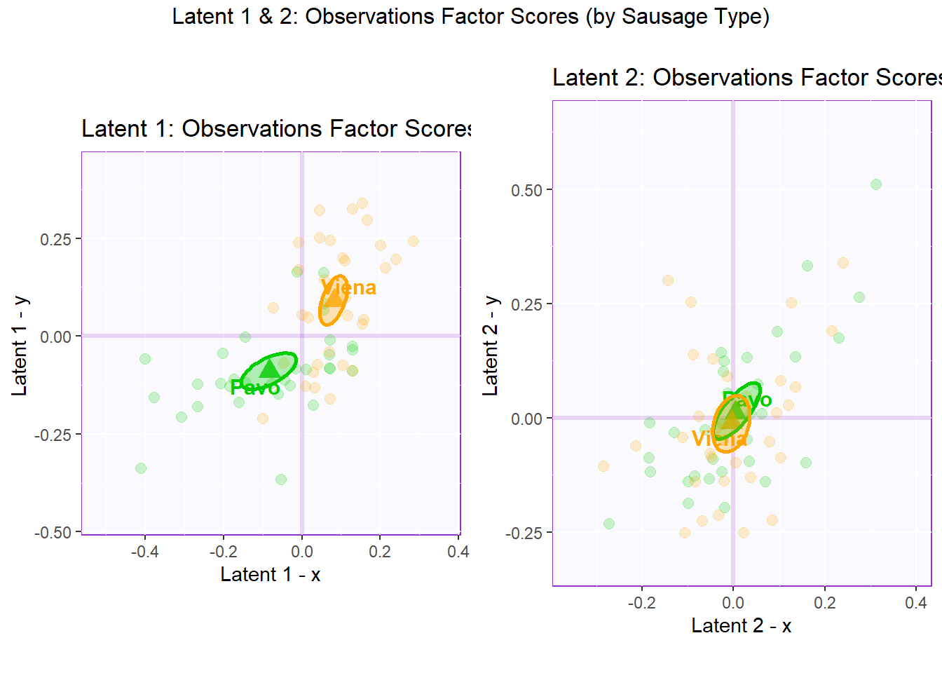
         labs(y = "Latent 1 - y ", x = "Latent 1 - x")

6.4.2.2 Latent 1 & 2: Observations Factor Scores (by Sausage Type)

Note that in PLSC’s observation factor scores map, X axis is formed by the Latent(n) X and Y axis is formed by the Latent(n) Y. Essentially, we are looking at the observations from the view of 1st latent variable of both tables. We can interpret observation factor scores by assessing the proximity of each data point and draw bootstrap (confidence intervals) to verify our results.

In the perspective of Sausage Type where the observations have Design = “Pavo” and “Viena”, we can see that there is a clear distinction between Pavo and Viena in latent 1. However, there is a lot more overlap between Pavo and Viena in latent 2.

## TableGrob (2 x 2) "arrange": 3 grobs
##   z     cells    name                 grob
## 1 1 (2-2,1-1) arrange       gtable[layout]
## 2 2 (2-2,2-2) arrange       gtable[layout]
## 3 3 (1-1,1-2) arrange text[GRID.text.6919]

6.4.2.3 Latent 1 & 2: Observations Factor Scores (by Product Type)

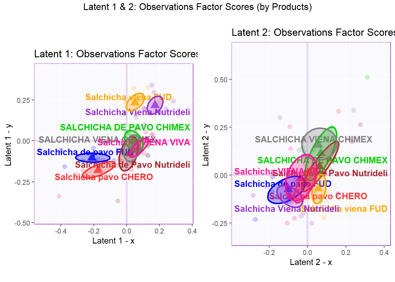
As established in the PCA section. The grouping option that is the clearest and gives the most insights is to group observations “by sausage type”. However, we will also draw observation factor scores by both Product Type and Panelist. The goal here is to look for any rating irregularity among products or panelits.

In the perspective of Product Type where the observations have Design = wk0$products (all 64 observations of 8 different products), we can see that there is no clear distinction between products in latent 1. We can also notice that 2 Viena sausages (FUD and Nutridelli) stays at the far end of latent 1 - Y while 2 Pavo sausages (FUD and Chero) stays at the far end of latent 1 - X. However, there is relatively more overlapping between products in latent 2.

## TableGrob (2 x 2) "arrange": 3 grobs
##   z     cells    name                 grob
## 1 1 (2-2,1-1) arrange       gtable[layout]
## 2 2 (2-2,2-2) arrange       gtable[layout]
## 3 3 (1-1,1-2) arrange text[GRID.text.7058]

6.4.2.4 Latent 1 & 2: Observations Factor Scores (by Panelists)

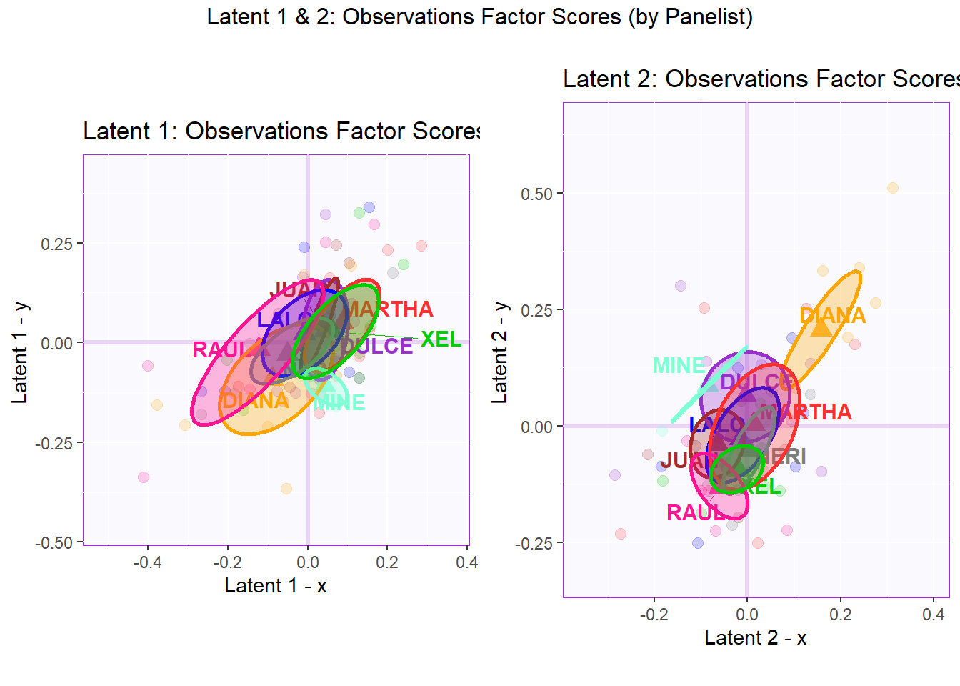
In the perspective of Panelist where the observations have Design = wk0$panelist (all 64 observations rated by 9 different panelist), we can see that there is no clear distinction between panelists in both latent 1 and 2. Note that not all panelist rated all 8 products, namely JUAN tested 7/8 products, MINE tested only 3/8 products, and RAUL tested only 6/8 products. We favor overlapping in this case because we want all panelists rate in a valid and consistent manner. We should look out for outlying confidence interval or those that are too large. We may have to control for this effect by scaling and centering on rows (per Panelist) if necessary.

In latent 1, we can notice that Raul has a pretty large confidence interval - this could mean that his ratings are not necessarily consistent when compared with other panelists (note that he only tested 6 of the products). In latent , we can notice XEL is a bit of an outlier with his/her ratings - confidence interval is not necessarily large but spread in a space with little overlapping.

## TableGrob (2 x 2) "arrange": 3 grobs
##   z     cells    name                 grob
## 1 1 (2-2,1-1) arrange       gtable[layout]
## 2 2 (2-2,2-2) arrange       gtable[layout]
## 3 3 (1-1,1-2) arrange text[GRID.text.7249]

6.4.3 Columns Factor Scores

Color:

#Color for all variables:
var <- colnames(sausage.processed)
var.color <- prettyGraphsColorSelection(n.colors = ncol(sausage.processed)) 

#Assign different colors to each set of variables:
var.color1 <- var.color[c(3:6,13)]
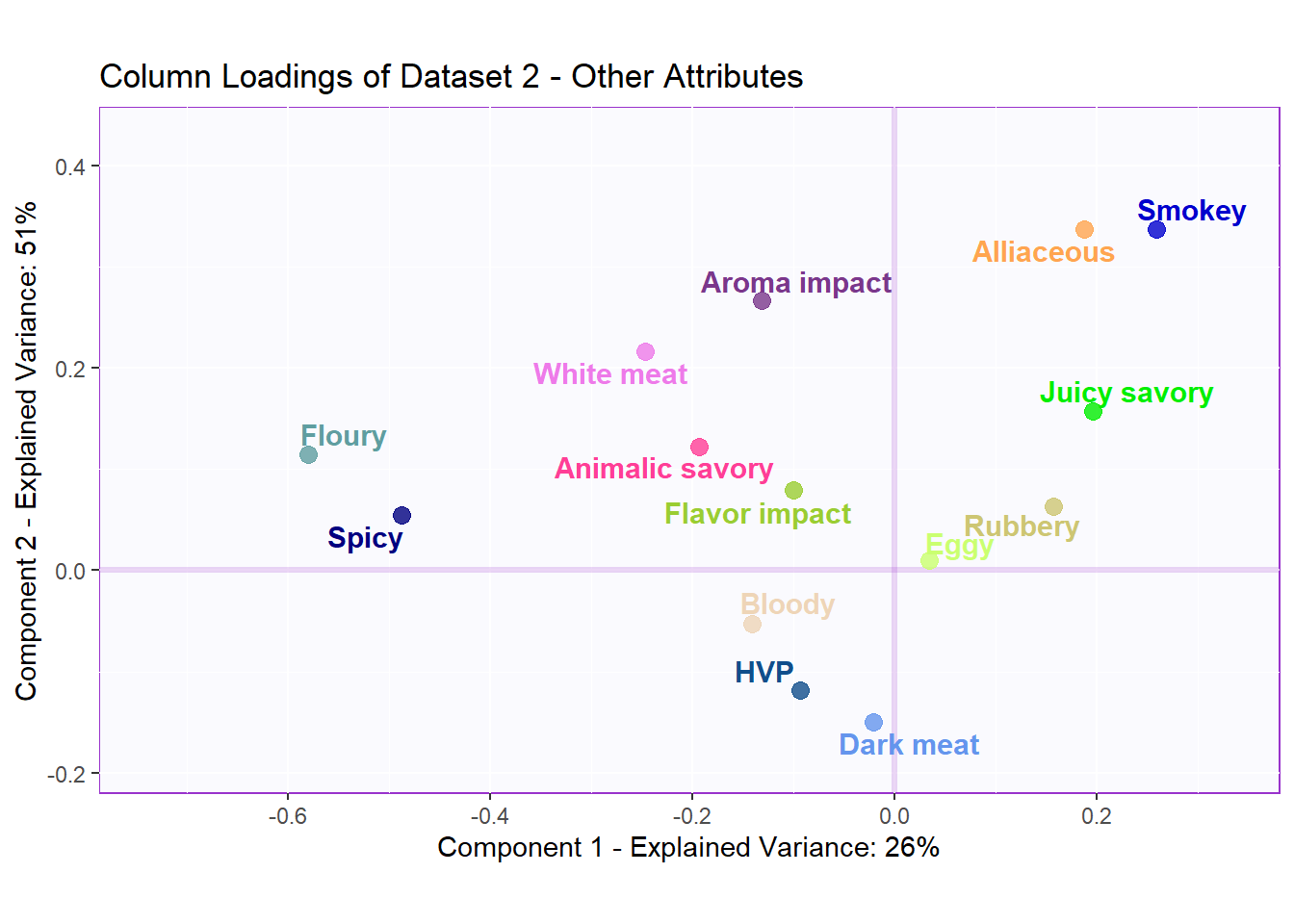
var.color2 <- var.color[-c(3:6,13)]

6.4.3.1 Latent 1 - The column loadings of the 1st component of X and Y.

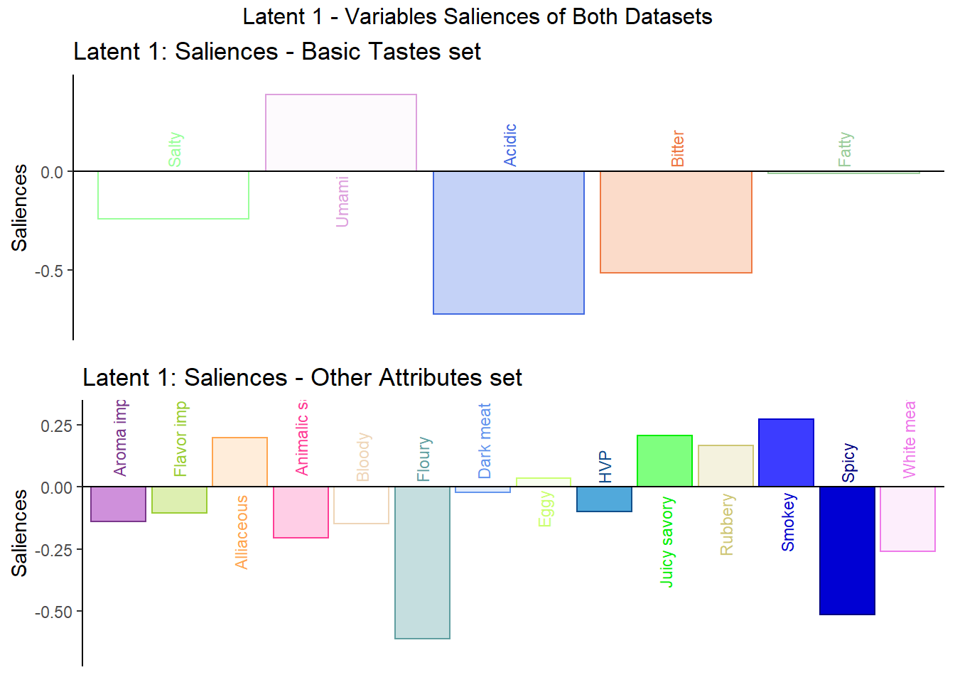
Saliences I-set:

P   <- pls$TExPosition.Data$pdq$p

plot3a <- PrettyBarPlot2(
  bootratio = P[,1], #change index to access other latents
  threshold = 0, 
  ylim = NULL, 
  color4bar = var.color1,
  color4ns = "gray75", 
  plotnames = TRUE, 
  main = 'Latent 1: Saliences - Basic Tastes set', 
  ylab = "Saliences")

Saliences J-set:

Q   <- pls$TExPosition.Data$pdq$q

plot3b <- PrettyBarPlot2(
  bootratio = Q[,1], #change index to access other latents
  threshold = 0, 
  ylim = NULL, 
  color4bar = var.color2,
  color4ns = "gray75", 
  plotnames = TRUE, 
  main = 'Latent 1: Saliences - Other Attributes set', 
  ylab = "Saliences")

Combine I-J of latent 1:

As mentioned above, Saliances is an inference tool that finds the square-root of eigenvalues in the singular values. The goal of saliances is to help find the relationship between variables on each latent and how good is the component. I think of this as the equivalence of Loadings in PCA.

Here in latent 1, we see that among the variables in data table 1 - Basic Tastes, Umami has an opposite effect with Salty, Acidic, and Bitter while Fatty has little effect overall. We can do the same for the variables in data table 2 - Other attributes to find the relationships there.

plot3 <- grid.arrange(
    plot3a,
    plot3b,
    ncol = 1,nrow = 2,
    top = "Latent 1 - Variables Saliences of Both Datasets"
  )

plot3

## TableGrob (3 x 1) "arrange": 3 grobs
##   z     cells    name                 grob
## 1 1 (2-2,1-1) arrange       gtable[layout]
## 2 2 (3-3,1-1) arrange       gtable[layout]
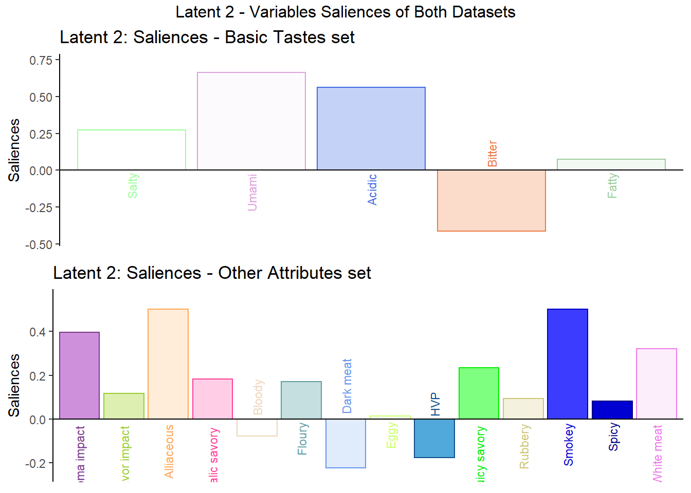
## 3 3 (1-1,1-1) arrange text[GRID.text.7386]

6.4.3.2 Latent 2 - The column loadings of the 2nd component of X and Y.

Here in latent 2, we see that among the variables in data table 1 - Basic Tastes, Bitter has an opposite effect with Salty, Umami, and Acidic while Fatty also has little effect overall. We can do the same for the variables in data table 2 - Other attributes to find the relationships there.

## TableGrob (3 x 1) "arrange": 3 grobs
##   z     cells    name                 grob
## 1 1 (2-2,1-1) arrange       gtable[layout]
## 2 2 (3-3,1-1) arrange       gtable[layout]
## 3 3 (1-1,1-1) arrange text[GRID.text.7451]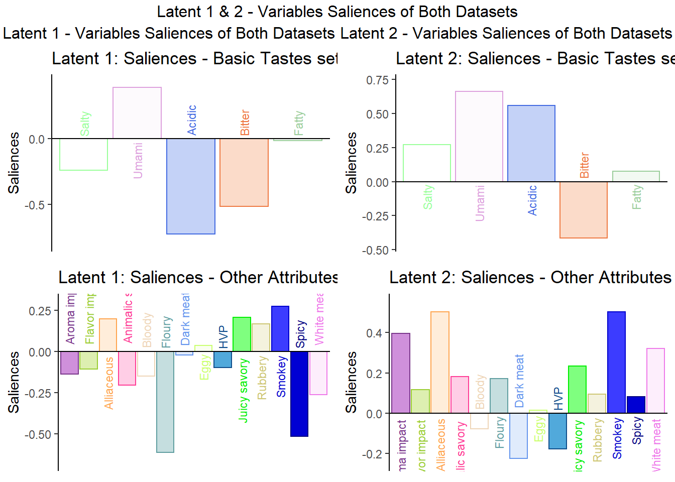

## TableGrob (2 x 2) "arrange": 3 grobs
##   z     cells    name                 grob
## 1 1 (2-2,1-1) arrange      gtable[arrange]
## 2 2 (2-2,2-2) arrange      gtable[arrange]
## 3 3 (1-1,1-2) arrange text[GRID.text.7452]

6.4.3.3 Extra Column Plots

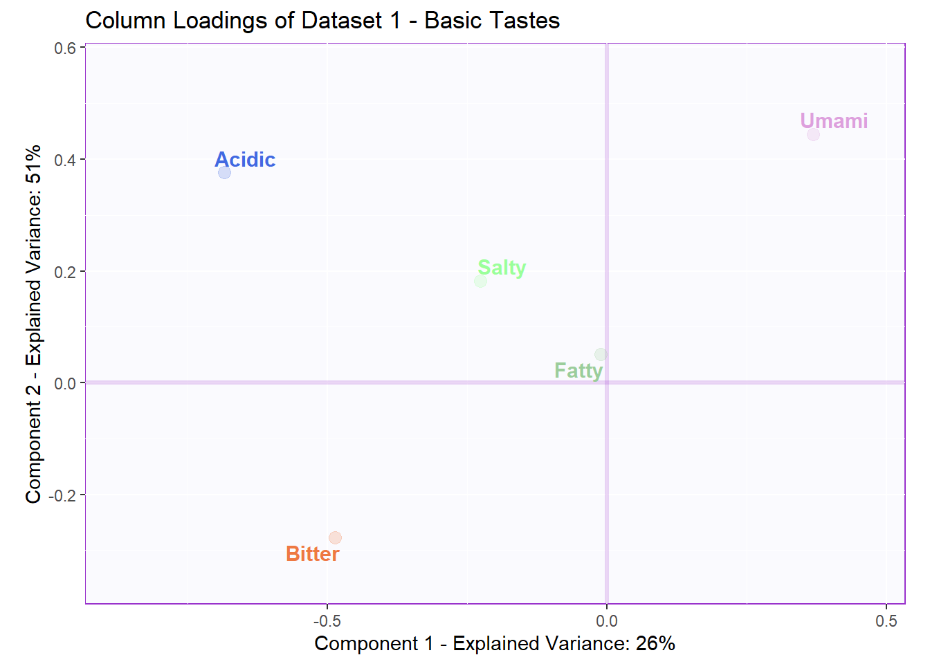
# the set of column of the first dataset (basic.tastes)
v1 <- pls$TExPosition.Data$fi
v2 <- pls$TExPosition.Data$fj

Here, I also present the typical loading map so that we can easily compare with the Salience Inference to see if we found any new insights. Overall, I think the Salience tests gives us novel information that clearly describes the relationships among the variables. We could only tell how similar the variables were using PCA loadings. Now, we can tell if the variables had a positive or negative relationship with each others using Salience.

6.4.4 Contributions and Bootstrap Ratios

We can use contribution to see which variable contributed above average for each latent. We can use Bootstrap Ratios to see essentially the same thing in that which variables are important for each latent by drawing conclusion from an infinite number of re-sampled populations (test everything to the extreme).

The variables that perform above average are colored and can be identied using the 2 plots below. Overall, we see relatively similar patterns when compared to PCA contribution and bootstrap ratios tests. The only difference is that each set of varaibles now have different averages and thus the effect of some varaibles are more pronounced now. We also see less effects from White Meat and Dark Meat

6.4.4.1 Contribution of Latent 1 and 2

# Contributions 
# Ctr I-set 
Fi   <- pls$TExPosition.Data$fi
ctri <- pls$TExPosition.Data$ci
signed.ctri <- ctri * sign(Fi)

# Ctr J-set 
Fj   <- pls$TExPosition.Data$fj
ctrj <- pls$TExPosition.Data$cj
signed.ctrj <- ctrj * sign(Fj)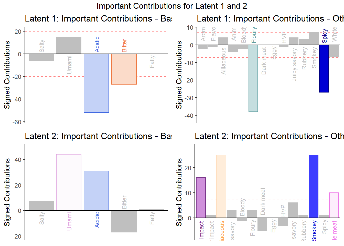

## TableGrob (3 x 2) "arrange": 5 grobs
##   z     cells    name                 grob
## 1 1 (2-2,1-1) arrange       gtable[layout]
## 2 2 (2-2,2-2) arrange       gtable[layout]
## 3 3 (3-3,1-1) arrange       gtable[layout]
## 4 4 (3-3,2-2) arrange       gtable[layout]
## 5 5 (1-1,1-2) arrange text[GRID.text.7743]

6.4.4.2 Bootstrap Ratio of Latent 1 and 2

Compute Bootstrap:

resBoot4PLSC <- Boot4PLSC(basic.taste, # First Data matrix 
                          others, # Second Data matrix
                          nIter = 1000, # How many iterations
                      Fi = pls$TExPosition.Data$fi,
                      Fj = pls$TExPosition.Data$fj,
                      nf2keep = 3,
                      critical.value = 2,
                      # To be implemented later
                      # has no effect currently
                      alphaLevel = .05)

BR.I <- resBoot4PLSC$bootRatios.i
BR.J <- resBoot4PLSC$bootRatios.j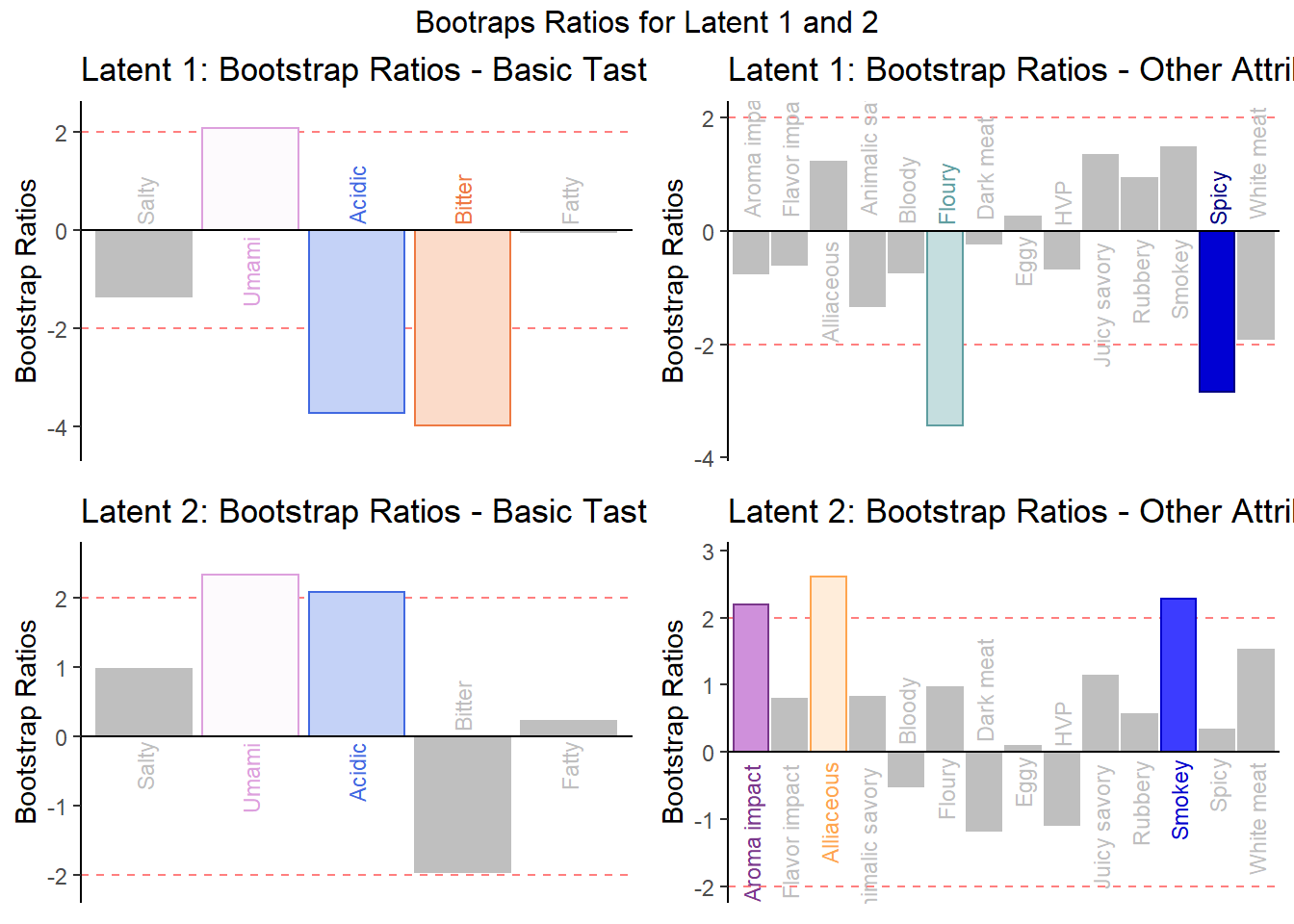

## TableGrob (3 x 2) "arrange": 5 grobs
##   z     cells    name                 grob
## 1 1 (2-2,1-1) arrange       gtable[layout]
## 2 2 (2-2,2-2) arrange       gtable[layout]
## 3 3 (3-3,1-1) arrange       gtable[layout]
## 4 4 (3-3,2-2) arrange       gtable[layout]
## 5 5 (1-1,1-2) arrange text[GRID.text.7872]