8.2 Data: Strawberry emotions in kids Colombia
Overview of the data:
Data:
75 consumers evaluated a set of 8 strawberry drinkable yogurts Mix of commercial strawberry products and strawberry prototypes The objective was to explore the emotions associated with strawberry yogurts
Consumer information:
N = 75 Bogotá, Colombia Men 50% Women 50% Age: 8 - 12 (50%) ; 13 - 20(50%). Database is the summary of the frequencies of all consumers selection Products were presented in a sequential monadic way (one at a time) Main question: How do you feel when you taste this product? Emotions were presented in a list, and consumers were able to choose as many emotions as they want
Load necessary packages:
library(readxl)                  #to read data the excel files
library(ggplot2)                 #to plot really pretty graphs
library(corrplot)                #to assess correlation and make correlation plots
library(PerformanceAnalytics)    #another cool package to look at correlation
library(PTCA4CATA)               #amazing package from Dr. Abdi to do support works 4 analysis
library(data4PCCAR)              #amazing package no.2 from Dr. Abdi to do PCA & CA
library(ExPosition)              #package for PCA calculations
library(InPosition)              #another package for PCA calculation that also include inference (BR, CI)
library(graphics)                #default on in R. Just making sure. For fine-tunings
library(dplyr)                   #for data manipulations
library(tidyverse)               #collection of vital packages
library(data.table)              #for data manipulation
library(knitr)                   #to make nice Rmarkdown including neat html tables
library(kableExtra)              #make scrollable tables
library(gridExtra)
library(grid)
library(ggplotify)               #these 3 helps combine plots
library(cowplot)                 #alternative to gridExtra, provides plot_grid
Load data:
#use readxl to read from excel files
data <- read_excel("data.xlsx")                #don't hard code location,
                                               #just direct to data file by name as long as it is in the same folder
a    <- kable(data)                            #taking a peak at our data
scroll_box(a, width = "100%", height = "200px")| Products | Happy | Pleasantly surprised | Refreshed | Calm | Comforted | Disgusted | Energetic | Joy | Interested | Irritated | Relaxed | Sad | Well-being |
|---|---|---|---|---|---|---|---|---|---|---|---|---|---|
| Nutriday Bebible | 3 | 1 | 10 | 1 | 5 | 2 | 4 | 13 | 2 | 2 | 4 | 2 | 1 |
| Alquería Niños | 5 | 2 | 7 | 5 | 2 | 3 | 3 | 8 | 4 | 2 | 8 | 1 | 2 |
| Yogo Yogo | 8 | 3 | 9 | 7 | 2 | 5 | 3 | 12 | 4 | 4 | 4 | 4 | 0 |
| Seedy strawberry | 8 | 0 | 16 | 7 | 1 | 0 | 1 | 17 | 8 | 4 | 4 | 3 | 1 |
| Jammy strawberry | 2 | 1 | 12 | 11 | 0 | 1 | 4 | 16 | 8 | 3 | 1 | 3 | 2 |
| Sweet strawberry | 9 | 3 | 9 | 9 | 1 | 3 | 2 | 8 | 8 | 1 | 3 | 3 | 2 |
| Candied strawberry | 3 | 1 | 12 | 9 | 1 | 0 | 0 | 12 | 6 | 0 | 4 | 1 | 4 |
| Fruity strawberry | 3 | 1 | 7 | 6 | 3 | 1 | 1 | 9 | 6 | 3 | 2 | 1 | 1 |
Process data:
Convert to data.frame and change product names into row names
#we will use wks to name and keep track of all version of data
wk0               <- as.data.frame(data)       # convert to data.frame
wk1               <- wk0                       # this version has product as rownames
rownames(wk1)     <- wk0$Products
wk1$Products      <- NULL
Assess data pattern:
Notes:
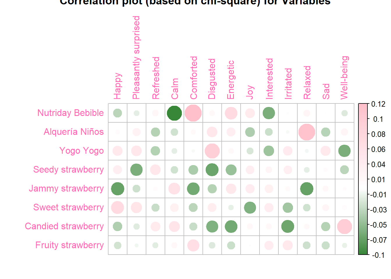
We will be using chisq.test() to perform chis-quare test for the data. Note that the ultility has a result component called $residual that contains the counts of the chi-square test. we will need to divide this by square root of sum of data to find the Inertia needed to do CA. This is because CA uses probabilities of contingency table. Based on R doc: residuals are the Pearson residuals, (observed - expected) / sqrt(expected).
# perform chi-square test on data
chi2    <-  chisq.test(wk1)

# Components of chi2: the chi-squares for each cell before we add them up to compute the chi2
Inertia.cells <- chi2$residuals / sqrt(sum(wk1))
Plot the inertia of cells:
corr <-  corrplot((Inertia.cells),
         is.cor = FALSE,
         tl.col = "hotpink",
         title = "Correlation plot (based on chi-square) for Variables",
         col=colorRampPalette(c("darkgreen","white","pink"))(200) )