Chapter 8 Introduction to Maps
This chapter shows examples of data visualization of the vaccination data with the use of vector maps.23 In the later sections we will also combine the Covid case data into the visualization. The work involves some data wrangling to format the vaccination and Covid case data with the vector map data frame.
This chapter is a simplified and updated version of our blog post.24
As mentioned in the write-up for Part II, it involves a combination of data frames with the necessary modifications.
We will need the following supporting packages. We have activated some in the earlier chapters.
library(ggplot2)
library(dplyr)
library(tidyverse)
library(tidyr)
library(readr)
library(sf)
library(maps)
library(patchwork)
library(leaflet)
8.1 Data Loading and Preparation
We use the data from here.25. We do some data cleaning to make the data usable for graphing. For those familiar with the tidyverse in R, most functions prefer to have data in long format.
Recall that the raw Malaysian vaccine dataset we downloaded in Chapter 1 is named vacn. We have saved it and will restore the saved vacn.rds file. (The full directory name may be different for our users.) To download the latest version run this command at the console line prompt; vacn <- read.csv("https://raw.githubusercontent.com/CITF-Malaysia/citf-public/main/vaccination/vax_state.csv")
# vacn <- read.csv("https://raw.githubusercontent.com/CITF-Malaysia/citf-public/main/vaccination/vax_state.csv")
# head(mys_vax)
mys1 <- readRDS("data/mys1.rds")
mysstates <- readRDS("data/mysstates.rds")
mysclusters <- readRDS("data/mysclusters.rds")
mysdeaths <- readRDS("data/mysdeaths.rds")
popn <- readRDS("data/popn.rds")
vacn <- readRDS("data/vacn.rds")
hospital <- readRDS("data/hospital.rds")
icu <- readRDS("data/icu.rds")
We check the columns or variables in vacn.
## 'data.frame':    3520 obs. of  20 variables:
##  $ date               : chr  "2021-02-24" "2021-02-24" "2021-02-24" "2021-02-24" ...
##  $ state              : chr  "Johor" "Kedah" "Kelantan" "Melaka" ...
##  $ daily_partial      : int  0 0 0 0 0 0 0 0 0 0 ...
##  $ daily_full         : int  0 0 0 0 0 0 0 0 0 0 ...
##  $ daily              : int  0 0 0 0 0 0 0 0 0 0 ...
##  $ daily_partial_child: int  0 0 0 0 0 0 0 0 0 0 ...
##  $ daily_full_child   : int  0 0 0 0 0 0 0 0 0 0 ...
##  $ cumul_partial      : int  0 0 0 0 0 0 0 0 0 0 ...
##  $ cumul_full         : int  0 0 0 0 0 0 0 0 0 0 ...
##  $ cumul              : int  0 0 0 0 0 0 0 0 0 0 ...
##  $ cumul_partial_child: int  0 0 0 0 0 0 0 0 0 0 ...
##  $ cumul_full_child   : int  0 0 0 0 0 0 0 0 0 0 ...
##  $ pfizer1            : int  0 0 0 0 0 0 0 0 0 0 ...
##  $ pfizer2            : int  0 0 0 0 0 0 0 0 0 0 ...
##  $ sinovac1           : int  0 0 0 0 0 0 0 0 0 0 ...
##  $ sinovac2           : int  0 0 0 0 0 0 0 0 0 0 ...
##  $ astra1             : int  0 0 0 0 0 0 0 0 0 0 ...
##  $ astra2             : int  0 0 0 0 0 0 0 0 0 0 ...
##  $ cansino            : int  0 0 0 0 0 0 0 0 0 0 ...
##  $ pending            : int  0 0 0 0 0 0 0 0 0 0 ...
There are significantly more columns in the vacn data frame from the first version.
We prepare the first data frame df1 by selecting some columns from vacn and then convert it into a long format using gather. We also make sure that date is in the proper format.
vacn %>%
  select(date,state,daily,
         cumul_partial,cumul_full,cumul,
         cumul_partial_child,cumul_full_child) %>%
  mutate(date = as.Date(date)) %>%
  gather(DoseType, Measure, 3:8) -> df1
head(df1)
## date state DoseType Measure
## 1 2021-02-24 Johor daily 0
## 2 2021-02-24 Kedah daily 0
## 3 2021-02-24 Kelantan daily 0
## 4 2021-02-24 Melaka daily 0
## 5 2021-02-24 Negeri Sembilan daily 0
## 6 2021-02-24 Pahang daily 08.1.1 Initial point plot
The input data for the number of vaccinations per day is shown in Figure 8.1.
df1 %>%
  filter(DoseType == "daily") %>%
  ggplot(aes(x = date, y = Measure, color=state, shape=state)) +
  geom_point() +
  scale_shape_manual(values=c(0,1,2,3,4,5,6,7,8,9,10,11,12,13,14,15)) +
  labs(title = "Daily Vaccination in Malaysia",
      subtitle = "Color by states")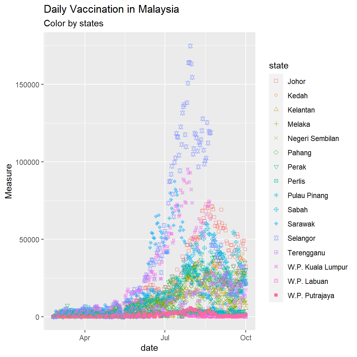
Figure 8.1: Point plot of Malaysia vaccination data
Figure 8.1 appears busy because there are too many (16) states. So we use facets as in Figure 8.2.
df1 %>%
  ggplot(aes(x = date, y = Measure, color=DoseType, shape=DoseType)) +
  geom_point() +
  labs(title = "Daily Vaccination in Malaysia",
       subtitle = "Color by Dose Type") +
  facet_wrap(~ state)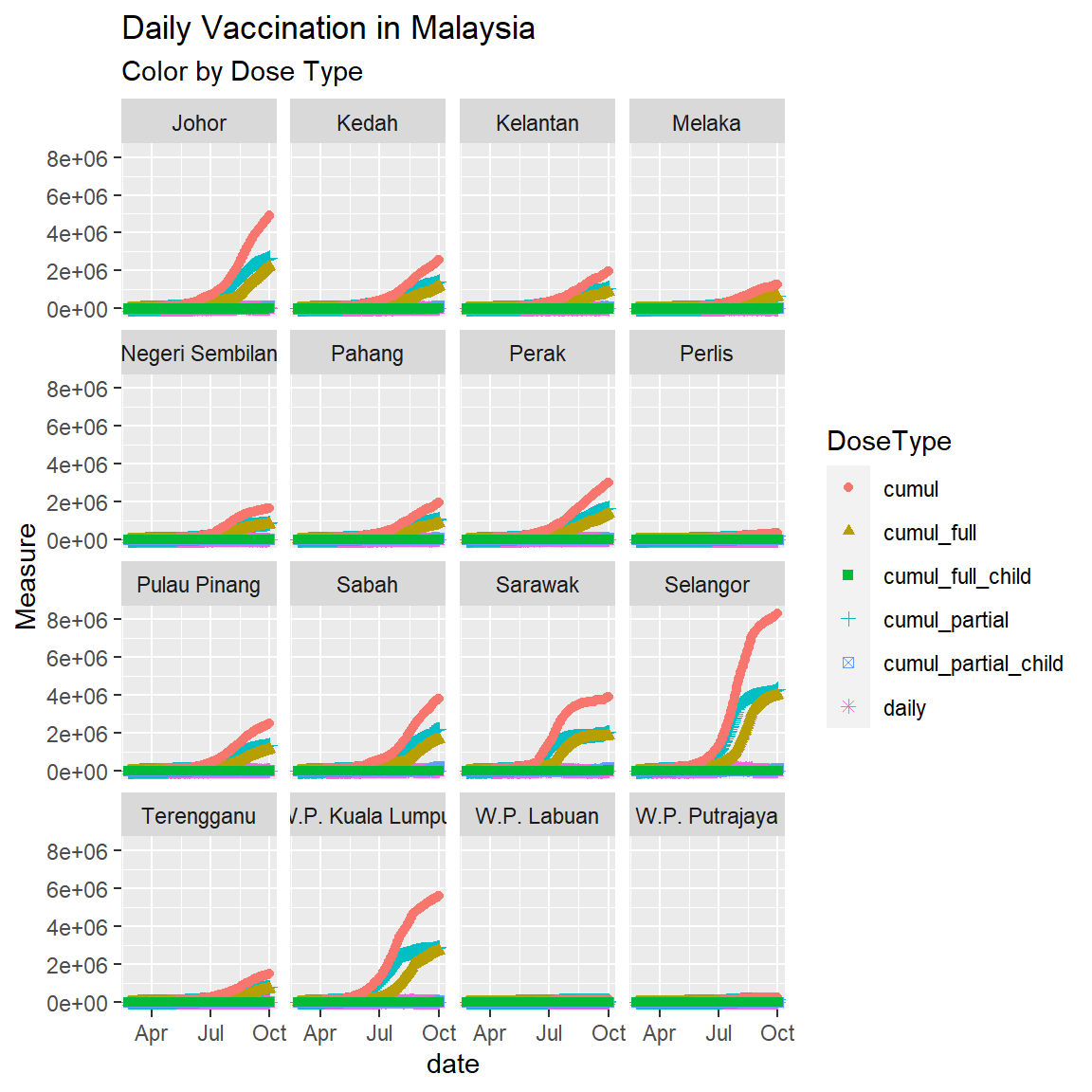
Figure 8.2: Point plot of vaccination data faceted by state
Figure 8.1 and Figure 8.2 show that Selangor, Sarawak, and W.P. Kuala Lumpur have increased the daily number of vaccinations. The simple point or line plot will not give us the same insight as if we plot it on a map. Child vaccination started only recently, so most of the data points are zero.
We will take some summary statistics and focus our analysis on these new measures. We convert state to the upper case since we plan to do a join later.
vacn$state <- toupper(vacn$state)
maxvacndate <- max(vacn$date)

vacn %>%
  group_by(state) %>%
  summarize(days_of_data = n(),
            avg_daily = mean(daily),
            med_daily = median(daily),
            min_daily = min(daily),
            max_daily = max(daily),
            dose1 = max(cumul_partial),
            dose2 = max(cumul_full),
            total = max(cumul)) -> vaxsum
We do a bubble plot to visualize the summary data instead of listing it. (Remember, this book is about visualization.)
vaxsum %>%
  ggplot(aes(x=avg_daily, y=max_daily, size=total, fill=state)) +
     geom_point(alpha=1, shape=21, color="black") +
     geom_text(data=vaxsum %>% filter(total >= 1000000),
               aes(label=state),
               size = 3,
               nudge_x = 0.25, nudge_y = 1,
               check_overlap = T) +
     labs(title = paste0("Bubble Plot of Daily Vaccination as of ",
                         maxvacndate),
          subtitle = "Highlight states with total vaccinations >= 1M",
          x = "Average Done",
          y = "Highest Done")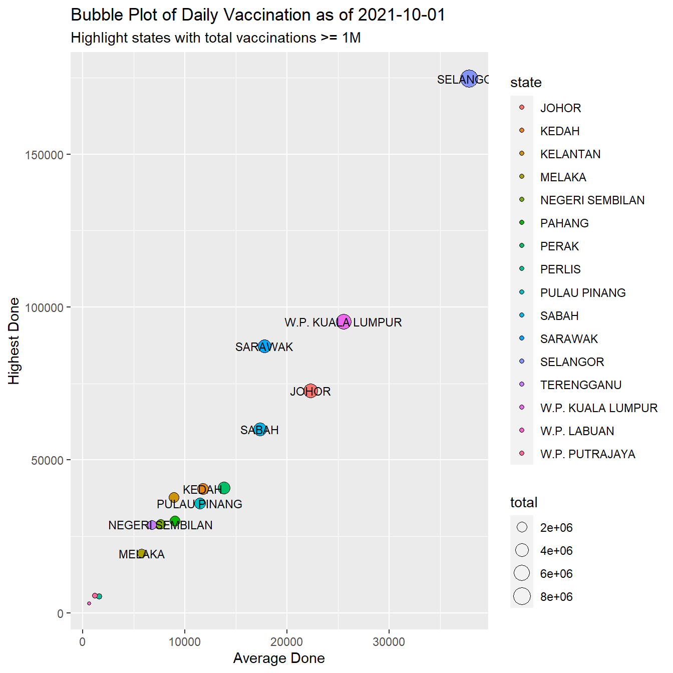
Figure 8.3: Vaccination summary by state
Figure 8.3 shows that SELANGOR, SARAWAK,and W.P. KUALA LUMPUR lead in both the average and highest numbers of vaccinations per day. They also lead in the total vaccinations. Note again that this bubble plot displays 3 variables.
8.2 Using Maps to Visualize Data
As a multi-platform, open-source language and environment for statistical computing and graphics, R has some good packages to support advanced geospatial statistics, modeling, and visualization. Spatial data and the broader topic of Geographic Information Systems (GIS) are huge subjects in R.26.
To visualize our Malaysian vaccination data and other Covid related data we need to
- find ready vector data models that represent the Malaysian map using points, lines, and polygons. These have discrete, well-defined borders, meaning that vector datasets usually have a high level of precision (but not necessarily accurate). This book uses the
sfpackage and thegeom_sffunction inggplotto work with vector data datasets. - prepare the vaccination data we want to visualize with the appropriate map vector data. This involves quite a bit of data wrangling using the
dplyrfunctions. - integrate with
ggplotso we can use other plotting functions by layering the graphs.geom_sfis a huge help.
We will learn all these by examples. We will explain some intricate details as we encounter specific problems.
8.2.1 Create and plot map of Malaysian states
To plot a map, we have to download the vector shapefile of districts and states in Malaysia.27
- Save and unzip the whole folder.
- Do not delete any of the files that have been unzipped.
- Then load the file
MYS_adm1.shp. (The directory notation may be different.) Again keep the other files in the same directory. - Rename columns to follow
vaxsum. This will facilitate thejoinoperations later. - Focus on the state data.
## Reading layer `MYS_adm1' from data source `F:\RProjects\CovidBook\data\MYS_adm1.shp' using driver `ESRI Shapefile'
## Simple feature collection with 13 features and 9 fields
## Geometry type: MULTIPOLYGON
## Dimension:     XY
## Bounding box:  xmin: 99.64072 ymin: 0.855001 xmax: 119.2697 ymax: 7.380556
## Geodetic CRS: WGS 84Using the state_sf data frame, we now simply plot the map using the geom_sf function.
state_sf %>%
   ggplot() +
   geom_sf(aes(geometry = geometry, fill = state)) +
   labs(title = "Map of all states in Malaysia",
subtitle = "Color by States") 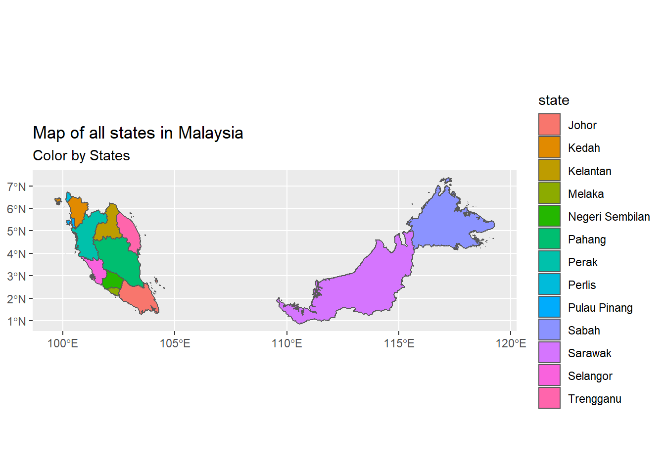
Figure 8.4: Map of all states in Malaysia
Comparing Figure 8.3 with Figure 8.4 shows that some of the states are not defined separately in the map. One option is to ignore these states for which we do not have the vector map readily defined in state_sf. We chose however to combine some of these states. We have to make the necessary adjustments to the data. Thus we
- correct some of the state names (like Trengganu).
- combine “SELANGOR”, “W.P. KUALA LUMPUR”, “W.P. PUTRAJAYA”
- combine “SABAH”, “W.P. LABUAN”
- add and adjust the state population data
First, we combine vaxsum with the state population data frame popn. We convert state to upper case in popn since we plan to do a join later.
## # A tibble: 16 x 13
##    state      days_of_data avg_daily med_daily min_daily max_daily  dose1  dose2
##    <chr>             <int>     <dbl>     <dbl>     <int>     <int>  <int>  <int>
##  1 JOHOR               220    22339.    13038          0     72702 2.69e6 2.23e6
##  2 KEDAH               220    11765.     7018          0     40576 1.43e6 1.16e6
##  3 KELANTAN            220     8924.     3484.         0     37709 1.09e6 8.78e5
##  4 MELAKA              220     5782.     2858.         0     19457 6.76e5 5.98e5
##  5 NEGERI SE~          220     7666.     3882.         0     28930 8.90e5 7.97e5
##  6 PAHANG              220     9010.     5068          0     30144 1.10e6 8.87e5
##  7 PERAK               220    13825.     8746          0     40898 1.68e6 1.37e6
##  8 PERLIS              220     1622.     1372          0      5343 1.91e5 1.66e5
##  9 PULAU PIN~          220    11500.     7688.         0     35875 1.38e6 1.15e6
## 10 SABAH               220    17380.    10696.         0     60003 2.22e6 1.68e6
## 11 SARAWAK             220    17829.     6135          0     87239 2.06e6 1.86e6
## 12 SELANGOR            220    37850.    18250.         0    174722 4.32e6 4.01e6
## 13 TERENGGANU          220     6794.     3762          0     28718 8.09e5 6.89e5
## 14 W.P. KUAL~          220    25557.    19664.         0     95232 2.90e6 2.72e6
## 15 W.P. LABU~          220      671.      378.         0      3061 7.99e4 6.76e4
## 16 W.P. PUTR~          220     1187.      726.         0      5744 1.36e5 1.25e5
## # ... with 5 more variables: total <int>, idxs <int>, pop <int>, pop_18 <int>,
## #   pop_60 <int>
Next we properly combine the data for “SELANGOR”, “W.P. KUALA LUMPUR”, “W.P. PUTRAJAYA” into “SELANGOR”.
vaxsum %>%
  filter(state %in% c("SELANGOR", "W.P. KUALA LUMPUR", "W.P. PUTRAJAYA")) %>%
  summarize(days_of_data = mean(days_of_data),
            avg_daily = mean(avg_daily),
            med_daily = median(med_daily),
            min_daily = min(min_daily),
            max_daily = max(max_daily),
            dose1 = sum(dose1),
            dose2 = sum(dose2),
            total = sum(total),
            pop = sum(pop),
            pop_18 = sum(pop_18),
            pop_60 = sum(pop_60)) %>%
  mutate(state = "SELANGOR") %>%
  select(state, everything()) -> tmp1
tmp1
## # A tibble: 1 x 12
## state days_of_data avg_daily med_daily min_daily max_daily dose1 dose2
## <chr> <dbl> <dbl> <dbl> <int> <int> <int> <int>
## 1 SELANGOR 220 21532. 18250. 0 174722 7356112 6856706
## # ... with 4 more variables: total <int>, pop <int>, pop_18 <int>, pop_60 <int>We now have changed the data for SELANGOR in vaxsum.
Next we repeat for “SABAH” and “W.P. LABUAN”.
vaxsum %>%
  filter(state %in% c("SABAH", "W.P. LABUAN")) %>%
  summarize(days_of_data = mean(days_of_data),
            avg_daily = mean(avg_daily),
            med_daily = median(med_daily),
            min_daily = min(min_daily),
            max_daily = max(max_daily),
            dose1 = sum(dose1),
            dose2 = sum(dose2),
            total = sum(total),
            pop = sum(pop),
            pop_18 = sum(pop_18),
            pop_60 = sum(pop_60)) %>%
  mutate(state = "SABAH") %>%
  select(state, everything()) -> tmp2
tmp2
## # A tibble: 1 x 12
## state days_of_data avg_daily med_daily min_daily max_daily dose1 dose2
## <chr> <dbl> <dbl> <dbl> <int> <int> <int> <int>
## 1 SABAH 220 9025. 5538. 0 60003 2298865 1748855
## # ... with 4 more variables: total <int>, pop <int>, pop_18 <int>, pop_60 <int>We have properly changed the data for SABAH in vaxsum.
Next, we filter out the old data for the five states and replace it with the new properly combined data for SELANGOR and SABAH. We unselect the column idxs in vaxsum so that the number of columns in vaxsum, tmp1 and tmp2 is the same for us to use the rbind function which simply binds the data frames by rows.
vaxsum %>%
  select(-idxs) %>%
  filter(!state %in% c("SELANGOR", "W.P. KUALA LUMPUR", "W.P. PUTRAJAYA",
                       "SABAH", "W.P. LABUAN")) %>%
  rbind(tmp1) %>%
  rbind(tmp2) -> vaxsum
vaxsum
## # A tibble: 13 x 12
## state days_of_data avg_daily med_daily min_daily max_daily dose1 dose2
## <chr> <dbl> <dbl> <dbl> <int> <int> <int> <int>
## 1 JOHOR 220 22339. 13038 0 72702 2.69e6 2.23e6
## 2 KEDAH 220 11765. 7018 0 40576 1.43e6 1.16e6
## 3 KELANTAN 220 8924. 3484. 0 37709 1.09e6 8.78e5
## 4 MELAKA 220 5782. 2858. 0 19457 6.76e5 5.98e5
## 5 NEGERI SE~ 220 7666. 3882. 0 28930 8.90e5 7.97e5
## 6 PAHANG 220 9010. 5068 0 30144 1.10e6 8.87e5
## 7 PERAK 220 13825. 8746 0 40898 1.68e6 1.37e6
## 8 PERLIS 220 1622. 1372 0 5343 1.91e5 1.66e5
## 9 PULAU PIN~ 220 11500. 7688. 0 35875 1.38e6 1.15e6
## 10 SARAWAK 220 17829. 6135 0 87239 2.06e6 1.86e6
## 11 TERENGGANU 220 6794. 3762 0 28718 8.09e5 6.89e5
## 12 SELANGOR 220 21532. 18250. 0 174722 7.36e6 6.86e6
## 13 SABAH 220 9025. 5538. 0 60003 2.30e6 1.75e6
## # ... with 4 more variables: total <int>, pop <int>, pop_18 <int>, pop_60 <int>Note that in all the steps we have kept the original vacn and popn data frames unchanged. We can always go back to the original data if need be.
We now have combined the summary vaccination data per state with the population data and combined the states for which we do not have the vector map data. We could have searched for the Malaysian vector map data that contains “W.P. KUALA LUMPUR”, “W.P. PUTRAJAYA”, and “W.P. LABUAN”, but that is another story. Along the way we have demonstrated compromises when we do not have all the data in the formats that we require. We have also shown some non-trivial examples of data wrangling.
Now we do a join with the vector map data frame state_sf. The key column for the join will be state.
- Make sure that all references to the state are in the same case.
- Remove some columns from
state_sfwith select(-c(1:4, 6:9))
vaxsum$state <- toupper(vaxsum$state)
state_sf$state <- toupper(state_sf$state)
state_sf$state[state_sf$state == "TRENGGANU"] <- "TERENGGANU"
# limit to only similar states in both data sets
intersect(vaxsum$state, state_sf$state) -> same_state
vaxsum %>% filter (state %in% same_state) -> vaxsum
# remove some columns
state_sf %>% select(-c(1:4, 6:9)) -> state_sf
# join
state_sf %>%
    left_join(vaxsum, by = "state") -> state_sf
state_sf
## Simple feature collection with 13 features and 12 fields
## Geometry type: MULTIPOLYGON
## Dimension: XY
## Bounding box: xmin: 99.64072 ymin: 0.855001 xmax: 119.2697 ymax: 7.380556
## Geodetic CRS: WGS 84
## First 10 features:
## state days_of_data avg_daily med_daily min_daily max_daily dose1
## 1 JOHOR 220 22339.291 13038.0 0 72702 2691154
## 2 KEDAH 220 11765.014 7018.0 0 40576 1428651
## 3 KELANTAN 220 8923.564 3483.5 0 37709 1086606
## 4 MELAKA 220 5781.855 2857.5 0 19457 676233
## 5 NEGERI SEMBILAN 220 7665.545 3882.5 0 28930 890157
## 6 PAHANG 220 9009.591 5068.0 0 30144 1097063
## 7 PERAK 220 13824.623 8746.0 0 40898 1682033
## 8 PERLIS 220 1621.936 1372.0 0 5343 191030
## 9 PULAU PINANG 220 11500.191 7687.5 0 35875 1380408
## 10 SABAH 220 9025.186 5537.5 0 60003 2298865
## dose2 total pop pop_18 pop_60 geometry
## 1 2226257 4914644 3781000 2711900 428700 MULTIPOLYGON (((103.4213 1....
## 2 1161747 2588303 2185100 1540600 272500 MULTIPOLYGON (((100.3289 5....
## 3 878049 1963184 1906700 1236200 194100 MULTIPOLYGON (((102.174 6.2...
## 4 597602 1272008 932700 677400 118500 MULTIPOLYGON (((102.335 2.0...
## 5 796611 1686420 1128800 814400 145000 MULTIPOLYGON (((101.7947 2....
## 6 887266 1982110 1678700 1175800 190200 MULTIPOLYGON (((103.4588 3....
## 7 1365287 3041417 2510300 1862700 397300 MULTIPOLYGON (((100.1029 3....
## 8 166248 356826 254900 181200 35100 MULTIPOLYGON (((100.1244 6....
## 9 1151496 2530042 1773600 1367200 239200 MULTIPOLYGON (((100.1797 5....
## 10 1748855 3971082 4008100 2826900 246800 MULTIPOLYGON (((118.6294 4....Now the state_sf data frame has both the vector map data for the 13 states and the associated vaccination summary data. We just plot the average daily vaccination and total vaccinations to date. We can easily repeat for the other statistics.
Note that %in% returns a logical vector of TRUE and FALSE. To negate it, we can use ! in front of the logical statement.
For Figure 8.5, we create two separate plots and combine them using the package cowplot.
state_sf %>%
    ggplot() +
    geom_sf(aes(geometry = geometry, fill = avg_daily)) +
# Everything past this point is only formatting:
    scale_fill_gradient2(low = "green",
                         mid = "yellow",
                         high = "red",
                         midpoint = 0,
                         space = "Lab",
                         na.value = "grey80",
                         guide = "colourbar",
                         aesthetics = "fill") +
    theme_void() +
    labs(title = paste0("Average daily vaccinations as of ", maxvacndate)) -> p1

state_sf %>%
    ggplot() +
    geom_sf(aes(geometry = geometry, fill = total)) +
# Everything past this point is only formatting:
    scale_fill_gradient2(low = "green",
                         mid = "yellow",
                         high = "red",
                         midpoint = 0,
                         space = "Lab",
                         na.value = "grey80",
                         guide = "colourbar",
                         aesthetics = "fill") +
    theme_void() +
    labs(title = paste0("Total Vaccination as of ", maxvacndate)) -> p2

cowplot::plot_grid(
     p1,
     p2,
     ncol = 1)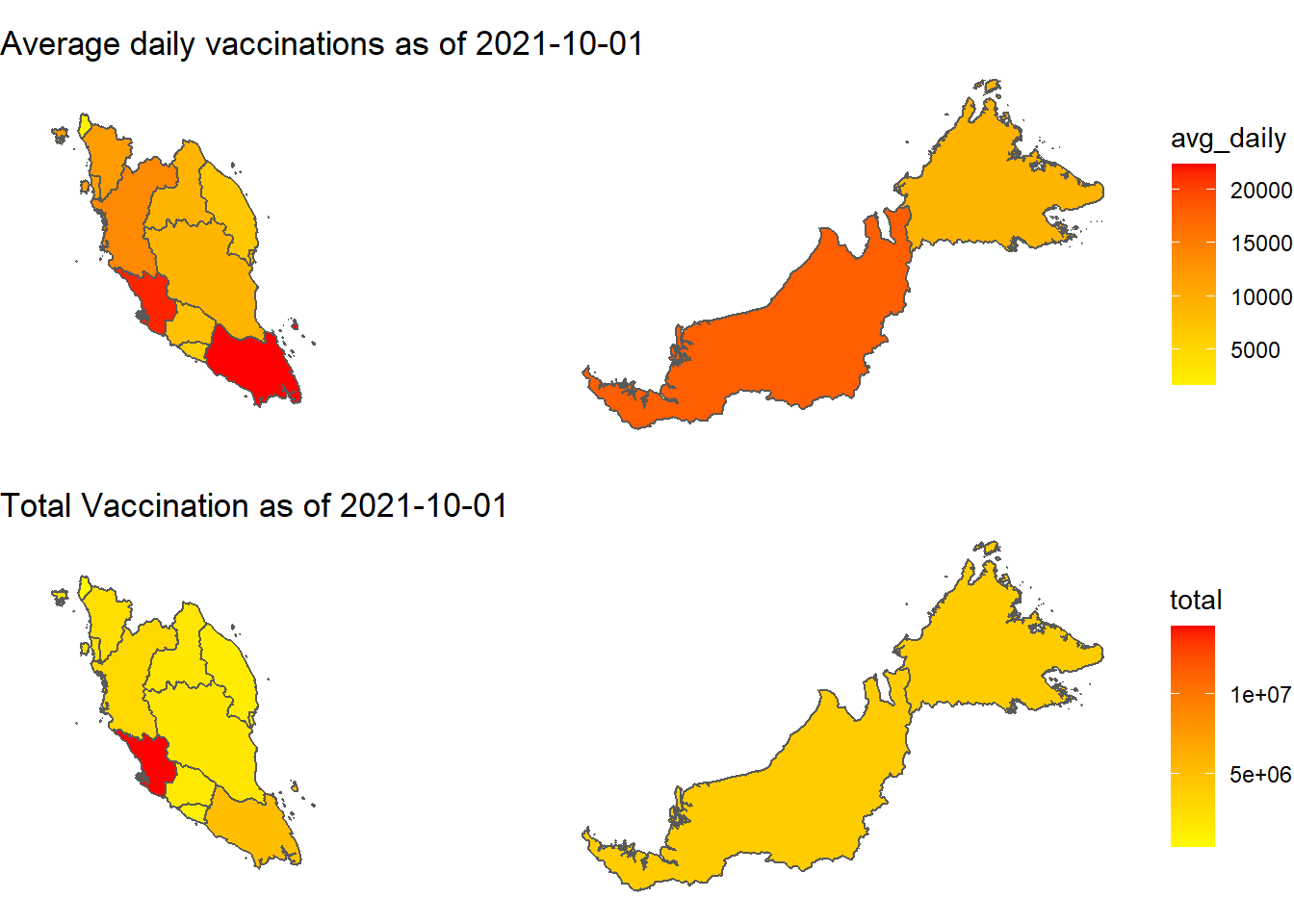
Figure 8.5: Vaccination by states
Figure 8.5 reconfirms the two states where vaccination is most advanced in terms of the numbers. Figure 8.8 however shows that this does not match with the Covid cases per state. It raises some questions on the planning of the Malaysian vaccination program.
Next we plot the population per state and the vaccination per population. We combine 3 separate plots. We use the pop column for the total population per state.
state_sf %>%
    ggplot() +
    geom_sf(aes(geometry = geometry, fill = pop)) +
# Everything past this point is only formatting:
    scale_fill_gradient2(low = "green",
                         mid = "yellow",
                         high = "red",
                         midpoint = 0,
                         space = "Lab",
                         na.value = "grey80",
                         guide = "colourbar",
                         aesthetics = "fill") +
    theme_void() +
    labs(title = "Population") -> p3

state_sf %>%
  mutate(vaccinated = (dose1/pop)*100) %>%
    ggplot() +
    geom_sf(aes(geometry = geometry, fill = vaccinated)) +
# Everything past this point is only formatting:
    scale_fill_gradient2(low = "green",
                         mid = "yellow",
                         high = "red",
                         midpoint = 0,
                         space = "Lab",
                         na.value = "grey80",
                         guide = "colourbar",
                         aesthetics = "fill") +
    theme_void() +
    labs(title = paste0("Percent partially vaccinated as of ",
                        maxvacndate)) -> p4

state_sf %>%
  mutate(vaccinated = (dose2/pop)*100) %>%
    ggplot() +
    geom_sf(aes(geometry = geometry, fill = vaccinated)) +
    scale_fill_gradient2(low = "green",
                         mid = "yellow",
                         high = "red",
                         midpoint = 0,
                         space = "Lab",
                         na.value = "grey80",
                         guide = "colourbar",
                         aesthetics = "fill") +
    theme_void() +
    labs(title = paste0("Percent fully vaccinated as of ",
                        maxvacndate)) -> p5

cowplot::plot_grid(
     p3,
     p4,
     p5, ncol = 1)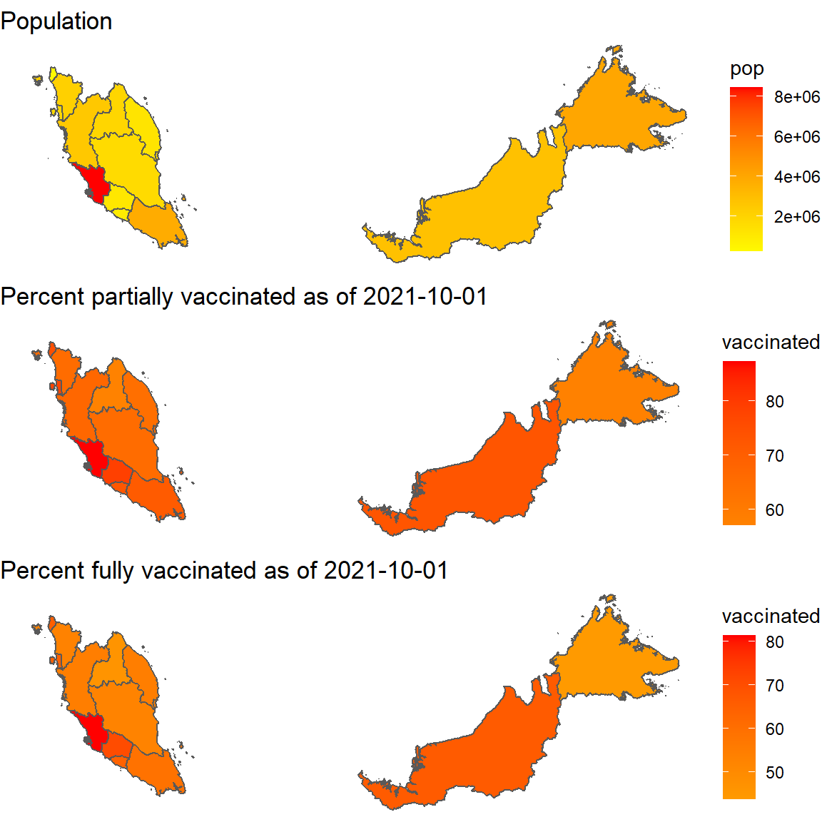
Figure 8.6: Map of population and percent vaccinated per state
All states have crossed the 50% fully vaccinated population as per 2021-10-01.
We must now look at the cases data and compare the maps visually.
8.3 Integrate with Covid case data
We now integrate with the Covid case data in mysstates data frame for which we now have the luxury to chose the point data as well as the various rolling averages that we calculated in Chapter 7. (We have progressed quite well from the raw data.)
We will take some summary statistics and focus our analysis on these new measures.
- Convert
stateto the upper case since we want to do a join later
mysstates$state <- toupper(mysstates$state)
maxcasedate <- max(mysstates$date)

mysstates %>%
  group_by(state) %>%
  summarize(avg_new = mean(cases_new),
            med_new = median(cases_new),
            lo_new = min(cases_new),
            hi_new = max(cases_new)) -> state_cases
We do a bubble plot of the summary data instead of displaying it.
state_cases %>%
  ggplot(aes(x=avg_new, y=hi_new, size=med_new, fill=state)) +
     geom_point(alpha=1, shape=21, color="black") +
     geom_text(data=state_cases %>% filter(med_new >= 50),
               aes(label=state),
               size = 3,
               nudge_x = 0.25, nudge_y = 1,
               check_overlap = T) +
     labs(title = paste0("Bubble Plot of Daily Covid cases as of ",
                         maxcasedate),
          subtitle = "Highlight states with median new cases >= 50",
          x = "Average Daily Case",
          y = "Highest Daily Case")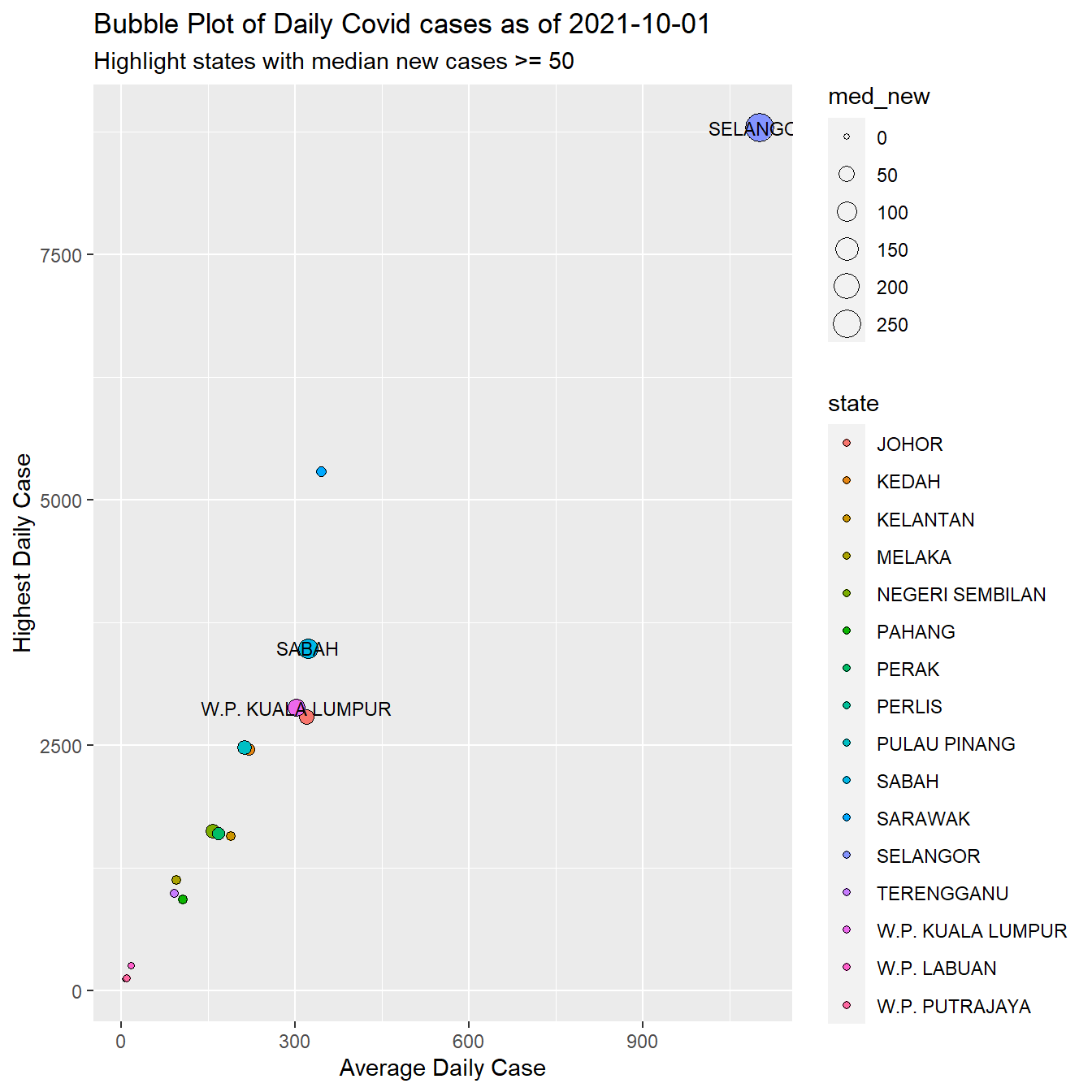
Figure 8.7: New daily case summary by state
By far, SELANGOR has the highest number of new cases per day on all the summary statistics we calculated. It is interesting to see where SARAWAK stands on the Covid cases (as compared to the vaccination data).
Next, we combine some of the case data to match the states defined in our map, Figure 8.4. This is the same process when we handled the vaxsum data frame.
state_cases %>%
  filter(state %in% c("SELANGOR", "W.P. KUALA LUMPUR", "W.P. PUTRAJAYA")) %>%
  summarize(avg_new = mean(avg_new),
            med_new = median(med_new),
            lo_new = min(lo_new),
            hi_new = max(hi_new)) %>%
  mutate(state = "SELANGOR") %>%
  select(state, everything()) -> tmp1
tmp1
## # A tibble: 1 x 5
## state avg_new med_new lo_new hi_new
## <chr> <dbl> <dbl> <dbl> <dbl>
## 1 SELANGOR 472. 68 0 8792state_cases %>%
filter(state %in% c("SABAH", "W.P. LABUAN")) %>%
summarize(avg_new = mean(avg_new),
med_new = median(med_new),
lo_new = min(lo_new),
hi_new = max(hi_new)) %>%
mutate(state = "SABAH") %>%
select(state, everything()) -> tmp2
tmp2## # A tibble: 1 x 5
## state avg_new med_new lo_new hi_new
## <chr> <dbl> <dbl> <dbl> <dbl>
## 1 SABAH 169. 49.8 0 3487Now we filter out the five states from state_cases and then add SELANGOR and SABAH with the modified data.
state_cases <- state_cases %>%
  filter(!state %in% c("SELANGOR", "W.P. KUALA LUMPUR", "W.P. PUTRAJAYA",
                   "SABAH", "W.P. LABUAN")) %>%
  rbind(tmp1) %>%
  rbind(tmp2)
state_cases
## # A tibble: 13 x 5
## state avg_new med_new lo_new hi_new
## <chr> <dbl> <dbl> <dbl> <dbl>
## 1 JOHOR 320. 44.5 0 2785
## 2 KEDAH 220. 16 0 2455
## 3 KELANTAN 189. 6.5 0 1573
## 4 MELAKA 95.3 5 0 1120
## 5 NEGERI SEMBILAN 158. 33 0 1619
## 6 PAHANG 106. 6 0 926
## 7 PERAK 168. 24 0 1596
## 8 PERLIS 6.45 0 0 113
## 9 PULAU PINANG 213. 35 0 2474
## 10 SARAWAK 344. 9.5 0 5291
## 11 TERENGGANU 91.5 3 0 993
## 12 SELANGOR 472. 68 0 8792
## 13 SABAH 169. 49.8 0 3487Now we have 13 states for both state_cases and state_sf (which also has the vaccination data). We join state_cases to state_sf.
Now we can just simply reuse the code for Figure 8.5 and Figure 8.6 by changing the fill option in geom_sf. (Best programming practices actually require us to write a function for re-usable code, but we intend to show the full steps here. We will introduce user-defined functions later.) We increase fig.height=10 since we will combine 5 plots.
state_sf %>%
    ggplot() +
    geom_sf(aes(geometry = geometry, fill = avg_new)) +
    scale_fill_gradient2(low = "green",
                         mid = "yellow",
                         high = "red",
                         midpoint = 0,
                         space = "Lab",
                         na.value = "grey80",
                         guide = "colourbar",
                         aesthetics = "fill") +
    theme_void() +
    labs(title = "Average new cases per day") -> p6

state_sf %>%
  mutate(avg_per_pop = (avg_new/pop)*100) %>%
    ggplot() +
    geom_sf(aes(geometry = geometry, fill = avg_per_pop)) +
    scale_fill_gradient2(low = "green",
                         mid = "yellow",
                         high = "red",
                         midpoint = 0,
                         space = "Lab",
                         na.value = "grey80",
                         guide = "colourbar",
                         aesthetics = "fill") +
    theme_void() +
    labs(title = "Average new cases per day per population") -> p7

state_sf %>%
  mutate(vaccinated = (dose1/avg_new)) %>%
    ggplot() +
    geom_sf(aes(geometry = geometry, fill = vaccinated)) +
    scale_fill_gradient2(low = "green",
                         mid = "yellow",
                         high = "red",
                         midpoint = 0,
                         space = "Lab",
                         na.value = "grey80",
                         guide = "colourbar",
                         aesthetics = "fill") +
    theme_void() +
    labs(title = "Partial vaccination per average cases") -> p8

state_sf %>%
  mutate(vaccinated = (dose2/avg_new)) %>%
    ggplot() +
    geom_sf(aes(geometry = geometry, fill = vaccinated)) +
    scale_fill_gradient2(low = "green",
                         mid = "yellow",
                         high = "red",
                         midpoint = 0,
                         space = "Lab",
                         na.value = "grey80",
                         guide = "colourbar",
                         aesthetics = "fill") +
    theme_void() +
    labs(title = "Full vaccination per average cases") -> p9

cowplot::plot_grid(
     p6,
     p7,
     p5,
     p8,
     p9, ncol = 1)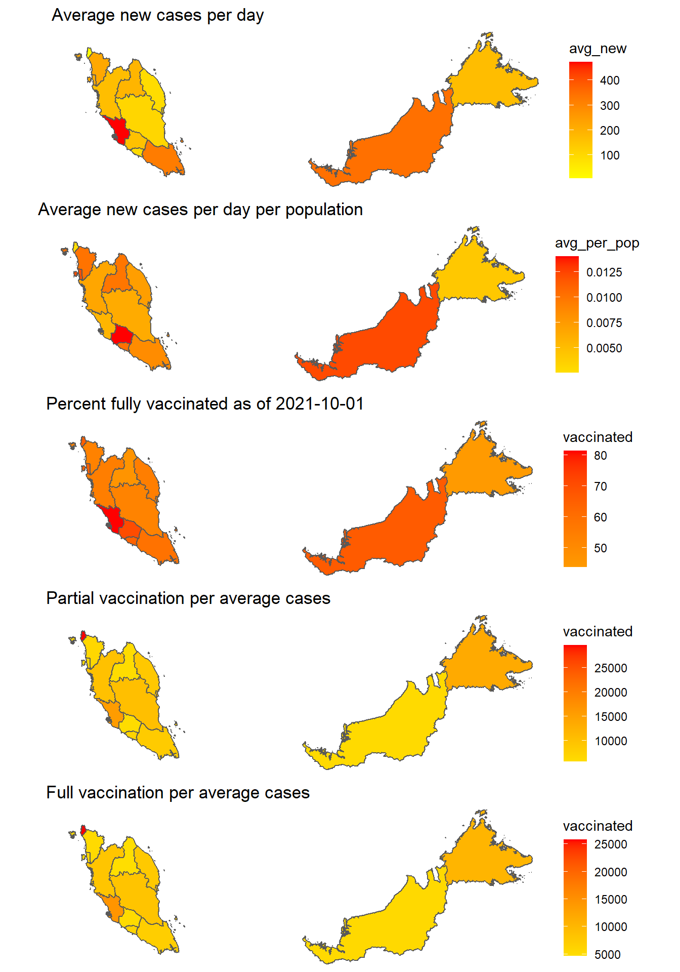
Figure 8.8: Covid cases and vaccination per state
Figure 8.8 raises some important issues and questions.
- MELAKA is the state with the highest number of daily cases (on average) per population. SELANGOR looks normal on this ratio. This ratio is rarely highlighted.
- For the low cases in SABAH, the vaccination rate is high. Perhaps more granular data at the district and mukim levels can give a better picture. The same applies to SARAWAK.
- PERLIS is a good candidate to start a phased exit from the current national lockdown. Perhaps an RCT (Randomized Control Trial) can be piloted there.
But the data does not show there is a clear strategy for the vaccination program except maybe for the categories of people like the frontliners, senior citizens, etc. Again we need more granular data to analyze.
8.4 Discussion
This chapter has illustrated how to combine the Malaysian Covid case and vaccination data and visualize some combinations of the data through vector maps. The various plots exhibited show the difference and added value when the ratios are incorporated in the analysis.
Figure 8.6 and Figure 8.8 really question the Malaysian vaccination program. What are its objectives? Is it to achieve a mass herd immunity for the nation? Is it to exit from the lockdown by state? Is it to control the rise in infections in the most problematic state, Selangor? The data to date shows a confusing picture.
Vaccination is a key intervention that is being considered in moving a country toward normalcy.28 Except for the supply of vaccines (which is improving), everything else related to the vaccination is in our own hands. But we must administer the vaccines with a clear purpose. We must do it to fit some exit strategy out of Covid. Right now, the current data does not show this. We need more granular data to answer some of the issues and questions raised.
Reference
Geocomputation with R, https://geocompr.robinlovelace.net/index.html↩︎
Malaysian Vaccination Data: Do we have a strategy?, https://rpubs.com/azmanH/788361↩︎
https://raw.githubusercontent.com/CITF-Malaysia/citf-public/9739fc10f85f2fbab06d98e9ce4ab43456c63fa3/vaccination/vax_state.csv↩︎
Geocomputation with R, a book on geographic data analysis, visualization and modeling, https://geocompr.robinlovelace.net/index.html↩︎