Chapter 7 Better Looking Graphs
In this final chapter of Part I, we learn how to improve the overall appearance of graphics made by ggplot2. We have mainly explored how our Covid data is processed and displayed; we have not been too concerned with things like fonts and background colors. The default fonts and colors are fine for quick data exploration, but customization can improve the clarity and attractiveness of a visual. We have mentioned that the theme functions provide control over the appearance of non-data elements. We have shown some examples of using theme in the previous chapters. Here we will show some of its other functions and workings.
We follow the flow of sub-topics from this simple structure.17
The mysdeaths data frame based on the deaths_state.csv file18 has some new columns/variables added compared to the earlier data.
date: yyyy-mm-dd format; data correct as of 1200hrs on that datestate: name of the statedeaths_new: deaths due to COVID-19 based on the date reported to the publicdeaths_bid: deaths due to COVID-19 which were brought-in dead based on the date reported to the public (a perfect subset of deaths_new)deaths_new_dod: deaths due to COVID-19 based on the date of deathdeaths_bid_dod: deaths due to COVID-19 which were brought-in dead based on the date of death (a perfect subset of deaths_new_dod)deaths_pvax: number of partially-vaccinated individuals who died due to COVID-19 based on the date of death (a perfect subset of deaths_new_dod), where “partially vaccinated” is defined as receiving at least 1 dose of a 2-dose vaccine at least 1 day prior to testing positive, or receiving the Cansino vaccine between 1-27 days before testing positive.deaths_fvax: number of fully-vaccinated who died due to COVID-19 based on the date of death (a perfect subset of deaths_new_dod), where “fully vaccinated” is defined as receiving the 2nd dose of a 2-dose vaccine at least 14 days prior to testing positive, or receiving the Cansino vaccine at least 28 days before testing positive.deaths_tat: median days between the date of death and date of the report for all deaths reported on the day
We will look at vaccinations, new cases, hospitalized Covid cases, and deaths more deeply in some chapters of Part III of this book. So perhaps we will benefit from some early visuals while learning how to customize the appearance of our visuals.
Many countries are trying to “live with the Covid”. This decision is close to the equilibrium solution in game theory.19 The equilibrium solution may be desirable or undesirable. Each party to the equilibrium solution may view the solution differently. For two warring parties; both sides may really desire to maintain the peace, or one (or both) side may view peace as an opportunity to regroup in order to pursue further hostilities. Accepting to live with Covid-19 is a form of the equilibrium solution. It is a fickle one because we’re aware of it, but not the virus, and it mutates.
Since we want to “live with the Covid”, we must keep track of the “deaths due to Covid” as the outcome measure or metric (we cannot decide to live with Covid and then more of us die due to Covid). Based on the columns in mysdeaths we will focus on
datestatedeaths_new_doddeaths_pvax: number of partially-vaccinated individuals who died due to COVID-19 based on the date of deathdeaths_fvax: number of fully-vaccinated who died due to COVID-19 based on the date of death
Note that deaths_pvax and deaths_fvax are perfect subsets of deaths_new_dod. We try to make this mundane chapter that discusses axes, colors, fonts and labels interesting and real by looking at Covid deaths. Hopefully, the data says that we are “living” in equilibrium with the Covid.
We filter and select from mysdeaths data frame based on some criteria.
- select only the five columns of interest
- filter from date of first vaccination in Malaysia, 24 Feb 202120
7.1 Axes
We have used the x-axis and y-axis to represent quantitative, categorical, and date values.
7.1.1 Quantitative
For quantitative variables, we have shown how to change the default scales using the scale_x_continuous or scale_y_continuous function for the axes in earlier chapters. We used the options
- breaks - a numeric vector of positions
- limits - a numeric vector with the minimum and maximum for the scale
We will show it again but using the updated mysdeaths data frame.
mysdeaths %>%
  filter(date >= as.Date("2021-02-24")) %>%
  select(date, state, deaths_new_dod, deaths_pvax, deaths_fvax) %>%
  filter(state == "Sarawak") %>%
  gather(key = "death_type", value = "deaths", 3:5) %>%
  ggplot(aes(x = as.Date(date),
             y = deaths,
             color = death_type)) +
  geom_line() +
  scale_y_continuous(breaks = seq(0, 20, 5),
                     limits = c(0, 20)) +
  labs(title = "Sarawak Covid Deaths by Category",
       subtitle = "Since 24 Feb 2021",
       x = "Date",
       y = "Deaths",
       color = "Death Category")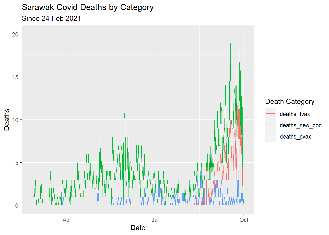
Figure 7.1: Types of Covid deaths for selected state
Next, we calculate the total deaths_new_dod, deaths_pvax, deaths_fvax for each state and visualize the 3 variables using a bubble plot.
mysdeaths %>%
  filter(date >= as.Date("2021-02-24")) %>%
  select(date, state, deaths_new_dod, deaths_pvax, deaths_fvax) %>%
  group_by(state) %>%
  summarize(totaldeaths = sum(deaths_new_dod),
            totalpvax = sum(deaths_pvax),
            totalfvax = sum(deaths_fvax)) %>%
  ggplot(aes(x = totalpvax,
             y = totalfvax,
             size = totaldeaths,
             fill = state)) +
  geom_point(alpha = 1, shape = 21, color= "black") +
  scale_x_continuous(breaks = seq(0, 2500, 100),
                     limits = c(0, 2500)) +
  scale_y_continuous(breaks = seq(0, 600, 50),
                     limits = c(0, 600)) +
  labs(title = "Covid Deaths Since Vaccination",
       subtitle = "Bubble size represents total deaths",
       x = "Deaths partially vaccinated",
       y = "Deaths fully vaccinated",
       fill = "State",
       size = "Total Deaths") +
  theme(axis.text.x = element_text(color = "darkblue", angle = 45, hjust = 1))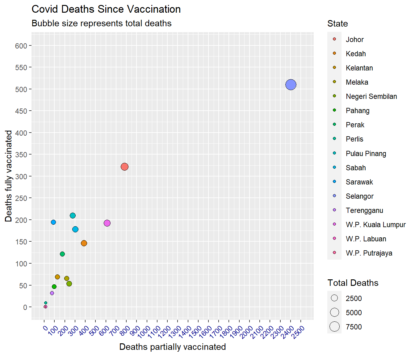
Figure 7.2: Bubble plot of Covid deaths
Obviously, we adjusted the parameters for scale_x_continuous, scale_y_continuous, and axis.text.x in Figure 7.2 after a few trials.
In Figure 7.3 we adjust the x-axis and y-axis to reflect the percentage of deaths that are partially and fully vaccinated. We are informed that deaths_pvax and deaths_fvax are perfect subsets of deaths_new_dod. Using percentages we can make a more direct visual comparison on the deaths despite being vaccinated. Note the use of label = scales::percent from the scales package.
mysdeaths %>%
  filter(date >= as.Date("2021-02-24")) %>%
  select(date, state, deaths_new_dod, deaths_pvax, deaths_fvax) %>%
  group_by(state) %>%
  summarize(totaldeaths = sum(deaths_new_dod),
            percentpvax = sum(deaths_pvax)/totaldeaths,
            percentfvax = sum(deaths_fvax)/totaldeaths) %>%
  ggplot(aes(x = percentpvax,
             y = percentfvax,
             size = totaldeaths,
             fill = state)) +
  geom_point(alpha = 1, shape = 21, color= "black") +
  scale_x_continuous(breaks = seq(0, 0.5, 0.05),
                     limits = c(0, 0.5),
                     label = scales::percent) +
  scale_y_continuous(breaks = seq(0, 0.5, 0.05),
                     limits = c(0, 0.5),
                     label = scales::percent) +
  geom_text(aes(label=state),
            size = 3,
            check_overlap = T) +
  labs(title = "Covid Deaths Since Vaccination",
       subtitle = "Bubble size represents total deaths",
       x = "% Deaths partially vaccinated",
       y = "% Deaths fully vaccinated",
       fill = "State",
       size = "Total Deaths") +
  theme(axis.text.x = element_text(color = "darkblue", angle = 45, hjust = 1))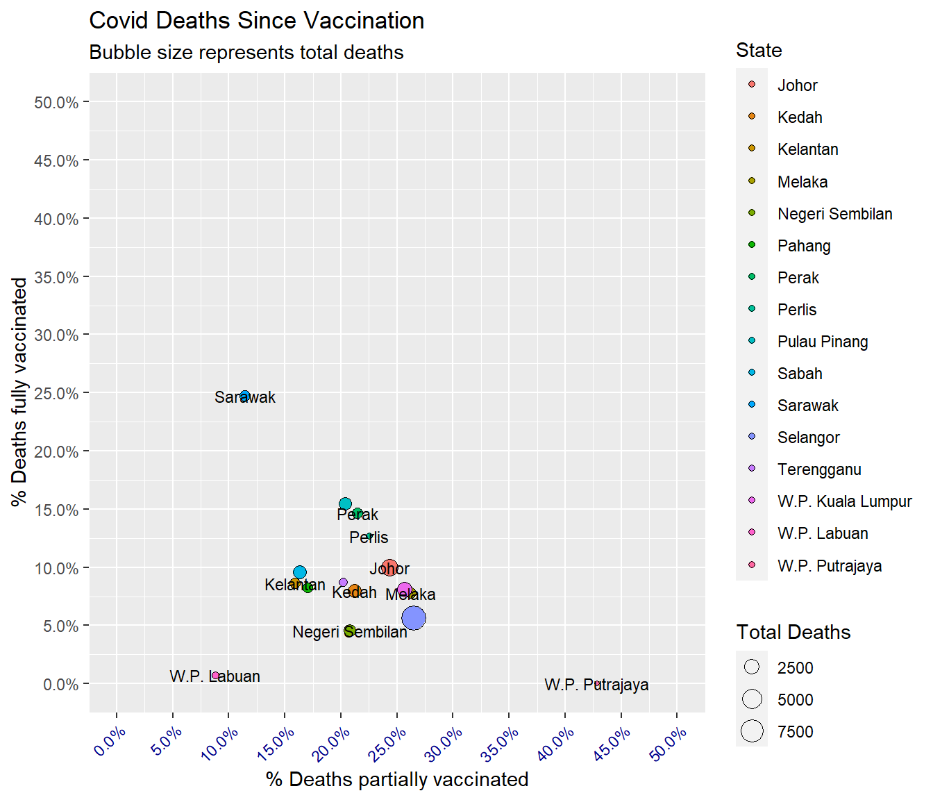
Figure 7.3: Bubble plot of Covid deaths
Figure 7.3 shows something different from Figure 7.2. There should be more concern about the death cases in Sarawak. The codes for Figure 7.3 are more since we have included more parameters to customize the graph.
7.1.2 Categorical
A categorical axis is modified using the scale_x_discrete or scale_y_discrete function. The options include
- limits - a character vector (the levels of the categorical variable in the desired order)
- labels - a character vector of labels (optional labels for these levels)
Levels define the set of allowed values.
mysdeaths %>%
  filter(date >= as.Date("2021-02-24")) %>%
  select(date, state, deaths_new_dod, deaths_bid_dod, deaths_pvax, deaths_fvax) %>%
  filter(state == "Sabah") %>%
  gather(key = "death_type", value = "deaths", 3:6) %>%
  group_by(death_type) %>%
  summarize(total = sum(deaths), .groups = 'drop') %>%
  ggplot(aes(x = death_type, y = total)) +
  geom_col(fill = "tomato2") +
  scale_x_discrete(limits = c("deaths_new_dod", "deaths_bid_dod", "deaths_fvax",
                              "deaths_pvax"),
                   labels = c("Deaths New DOD", "BID-DOD", "Full Vax",
                              "Partial Vax")) +
  labs(title = "Sabah Covid deaths by category",
       subtitle = "Since 24 Feb 2021",
       x = "Death Type",
       y = "Total Deaths")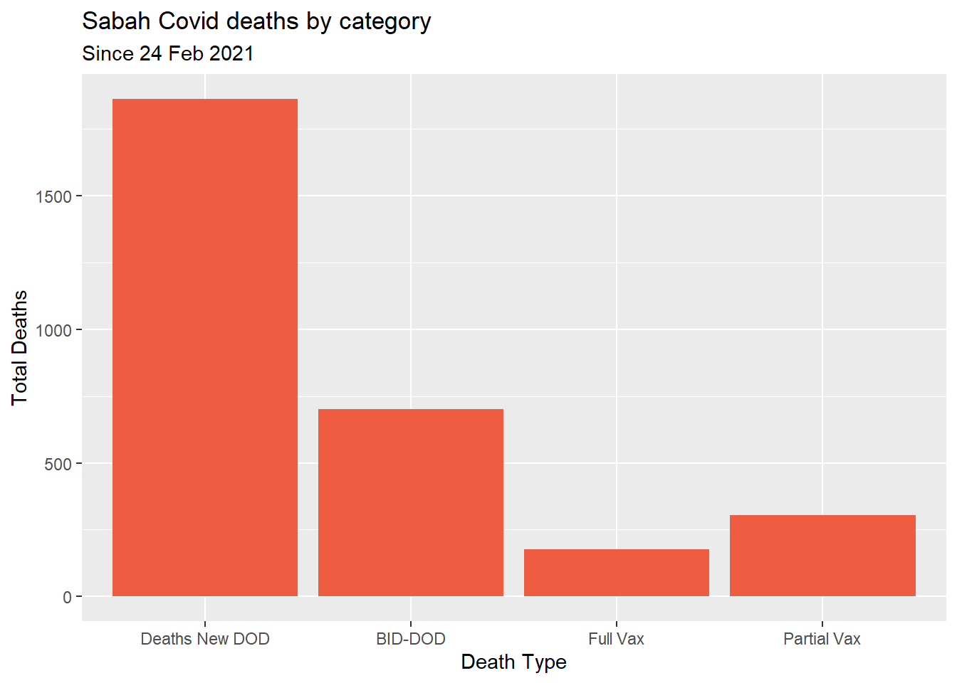
Figure 7.4: Types of Covid deaths for selected state
7.1.3 Date axes
We use the scale_x_date or scale_y_date function to change the date axis. The parameter date_breaks specifies the distance between breaks like “7 days” or “1 month”. date_labels specifies the format for the labels.
Some format specifications for date values are
- %d day as a number (0-31)
- %m month (00-12)
- %b abbreviated month like Jan
- %y 2-digit year like 21
- %Y 4-digit year like 2021
We use these to modify Figure 7.4 for state == "Selangor". We also use mutate to create better labels for displaying the types of Covid deaths.
mysdeaths %>%
  filter(date >= as.Date("2021-02-24")) %>%
  select(date, state, deaths_new_dod, deaths_pvax, deaths_fvax) %>%
  filter(state == "Selangor") %>%
  gather(key = "death_type", value = "deaths", 3:5) %>%
  mutate(death_type = case_when(
    death_type == "deaths_new_dod" ~ "1. New deaths",
    death_type == "deaths_pvax" ~ "2. Partial vax",
    death_type == "deaths_fvax" ~ "3. Full vax",
    TRUE ~ NA_character_)) %>%
  ggplot(aes(x = as.Date(date),
             y = deaths,
             color = death_type)) +
  geom_line() +
  scale_y_continuous(breaks = seq(0, 200, 10),
                     limits = c(0, 200)) +
  scale_x_date(date_breaks = "1 month",
               date_labels = "%b-%Y") +
  labs(title = "Selangor Covid Deaths by Category",
       subtitle = "Since 24 Feb 2021",
       x = "Date",
       y = "Deaths",
       color = "Death Category")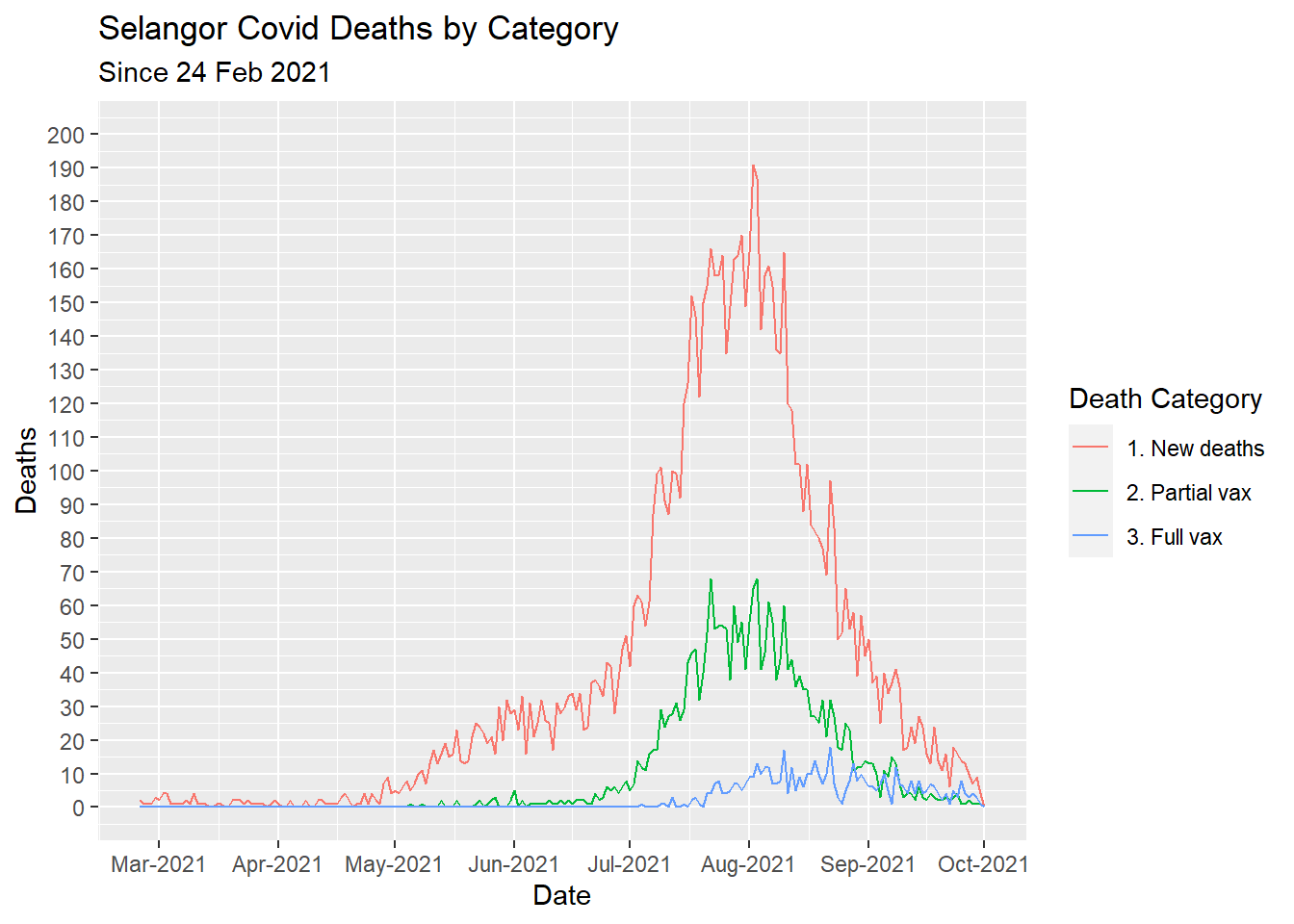
Figure 7.5: Types of Covid deaths for selected state
7.2 Colors
In the preceding chapters, we have shown many examples of specifying colors for points, lines, bars, areas, and text. We have also covered using colors to map the levels of a variable in the dataset. We purposely used the different color names in ggplot2 like “steelblue” and “tomato2” to see how it appears in the graphs. We also showed how to specify colors using hex codes.
We have also shown how to assign colors to the levels of a variable using the scale_color_manual for points and lines.
In the next example, we show how to use the scale_fill_manual function to manually specify the colors for bars and areas. We take the same summary approach as in Figure 7.4 but look at all the states.
mysdeaths %>%
  filter(date >= as.Date("2021-02-24")) %>%
  select(date, state, deaths_new_dod, deaths_bid_dod, deaths_pvax, deaths_fvax) %>%
  gather(key = "death_type", value = "deaths", 3:6) %>%
  group_by(state, death_type) %>%
  summarize(total = sum(deaths), .groups = 'drop') %>%
  ggplot(aes(x = state, y = total, fill = death_type)) +
  geom_col() +
  scale_fill_manual(values = c("red", "blue",
                               "green", "gold")) +
  labs(title = "Total Covid deaths by category",
       subtitle = "Since 24 Feb 2021",
       x = "Death Type",
       y = "Total Deaths",
       fill = "Death Category") +
  theme(axis.text.x = element_text(color = "darkblue", angle = 45, hjust = 1))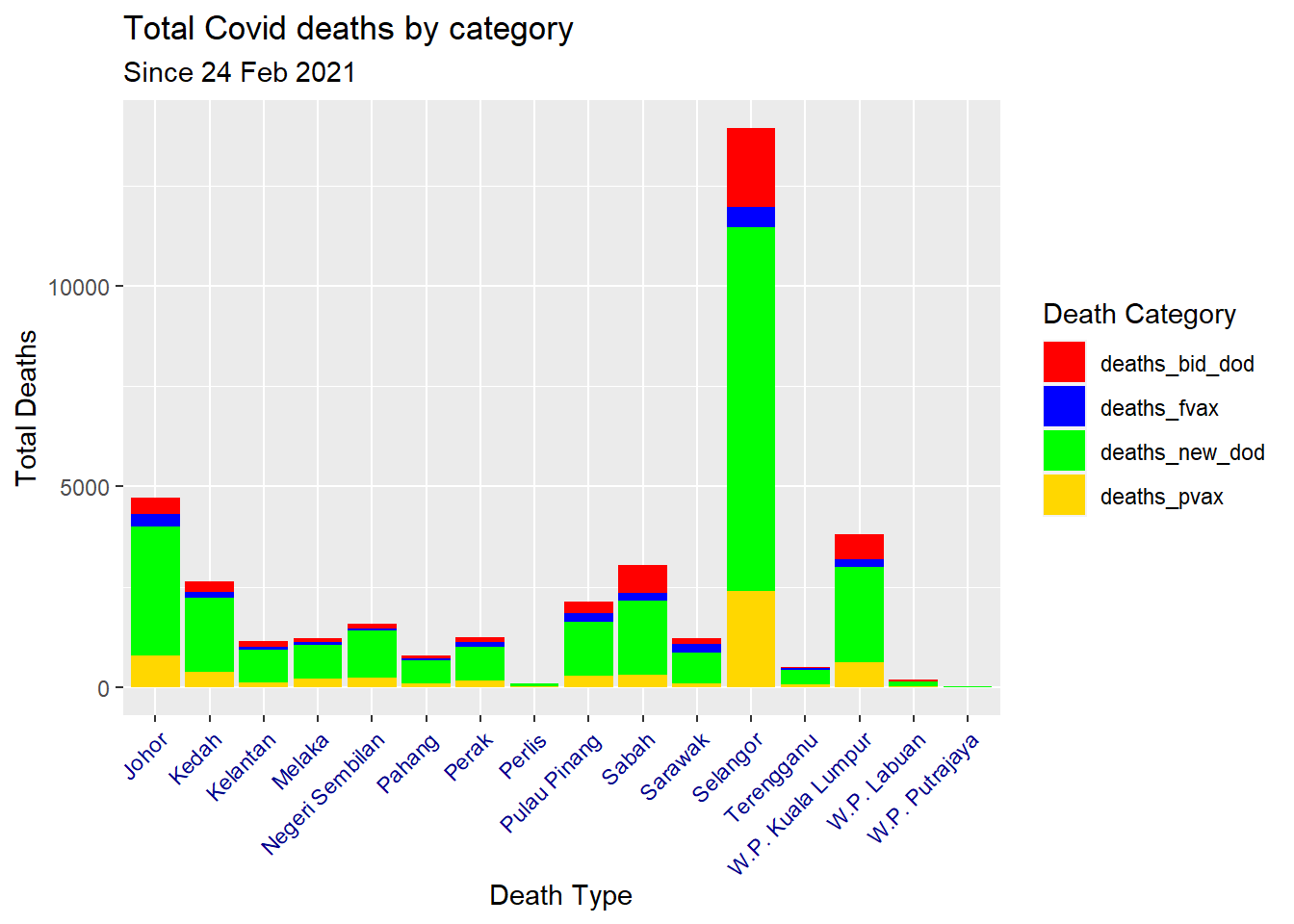
Figure 7.6: Types of Covid deaths for all states
The manual colors we chose for Figure 7.6 are for illustration. They do not look nice, so R has 657 built in color names. To see a list of names:
## [1] "white" "aliceblue" "antiquewhite"
## [4] "antiquewhite1" "antiquewhite2" "antiquewhite3"
## [7] "antiquewhite4" "aquamarine" "aquamarine1"
## [10] "aquamarine2" "aquamarine3" "aquamarine4"
## [13] "azure" "azure1" "azure2"
## [16] "azure3" "azure4" "beige"
## [19] "bisque" "bisque1" "bisque2"
## [22] "bisque3" "bisque4" "black"
## [25] "blanchedalmond" "blue" "blue1"
## [28] "blue2" "blue3" "blue4"
## [31] "blueviolet" "brown" "brown1"
## [34] "brown2" "brown3" "brown4"
## [37] "burlywood" "burlywood1" "burlywood2"
## [40] "burlywood3" "burlywood4" "cadetblue"
## [43] "cadetblue1" "cadetblue2" "cadetblue3"
## [46] "cadetblue4" "chartreuse" "chartreuse1"
## [49] "chartreuse2" "chartreuse3" "chartreuse4"
## [52] "chocolate" "chocolate1" "chocolate2"
## [55] "chocolate3" "chocolate4" "coral"
## [58] "coral1" "coral2" "coral3"
## [61] "coral4" "cornflowerblue" "cornsilk"
## [64] "cornsilk1" "cornsilk2" "cornsilk3"
## [67] "cornsilk4" "cyan" "cyan1"
## [70] "cyan2" "cyan3" "cyan4"
## [73] "darkblue" "darkcyan" "darkgoldenrod"
## [76] "darkgoldenrod1" "darkgoldenrod2" "darkgoldenrod3"
## [79] "darkgoldenrod4" "darkgray" "darkgreen"
## [82] "darkgrey" "darkkhaki" "darkmagenta"
## [85] "darkolivegreen" "darkolivegreen1" "darkolivegreen2"
## [88] "darkolivegreen3" "darkolivegreen4" "darkorange"
## [91] "darkorange1" "darkorange2" "darkorange3"
## [94] "darkorange4" "darkorchid" "darkorchid1"
## [97] "darkorchid2" "darkorchid3" "darkorchid4"
## [100] "darkred" "darksalmon" "darkseagreen"
## [103] "darkseagreen1" "darkseagreen2" "darkseagreen3"
## [106] "darkseagreen4" "darkslateblue" "darkslategray"
## [109] "darkslategray1" "darkslategray2" "darkslategray3"
## [112] "darkslategray4" "darkslategrey" "darkturquoise"
## [115] "darkviolet" "deeppink" "deeppink1"
## [118] "deeppink2" "deeppink3" "deeppink4"
## [121] "deepskyblue" "deepskyblue1" "deepskyblue2"
## [124] "deepskyblue3" "deepskyblue4" "dimgray"
## [127] "dimgrey" "dodgerblue" "dodgerblue1"
## [130] "dodgerblue2" "dodgerblue3" "dodgerblue4"
## [133] "firebrick" "firebrick1" "firebrick2"
## [136] "firebrick3" "firebrick4" "floralwhite"
## [139] "forestgreen" "gainsboro" "ghostwhite"
## [142] "gold" "gold1" "gold2"
## [145] "gold3" "gold4" "goldenrod"
## [148] "goldenrod1" "goldenrod2" "goldenrod3"
## [151] "goldenrod4" "gray" "gray0"
## [154] "gray1" "gray2" "gray3"
## [157] "gray4" "gray5" "gray6"
## [160] "gray7" "gray8" "gray9"
## [163] "gray10" "gray11" "gray12"
## [166] "gray13" "gray14" "gray15"
## [169] "gray16" "gray17" "gray18"
## [172] "gray19" "gray20" "gray21"
## [175] "gray22" "gray23" "gray24"
## [178] "gray25" "gray26" "gray27"
## [181] "gray28" "gray29" "gray30"
## [184] "gray31" "gray32" "gray33"
## [187] "gray34" "gray35" "gray36"
## [190] "gray37" "gray38" "gray39"
## [193] "gray40" "gray41" "gray42"
## [196] "gray43" "gray44" "gray45"
## [199] "gray46" "gray47" "gray48"
## [202] "gray49" "gray50" "gray51"
## [205] "gray52" "gray53" "gray54"
## [208] "gray55" "gray56" "gray57"
## [211] "gray58" "gray59" "gray60"
## [214] "gray61" "gray62" "gray63"
## [217] "gray64" "gray65" "gray66"
## [220] "gray67" "gray68" "gray69"
## [223] "gray70" "gray71" "gray72"
## [226] "gray73" "gray74" "gray75"
## [229] "gray76" "gray77" "gray78"
## [232] "gray79" "gray80" "gray81"
## [235] "gray82" "gray83" "gray84"
## [238] "gray85" "gray86" "gray87"
## [241] "gray88" "gray89" "gray90"
## [244] "gray91" "gray92" "gray93"
## [247] "gray94" "gray95" "gray96"
## [250] "gray97" "gray98" "gray99"
## [253] "gray100" "green" "green1"
## [256] "green2" "green3" "green4"
## [259] "greenyellow" "grey" "grey0"
## [262] "grey1" "grey2" "grey3"
## [265] "grey4" "grey5" "grey6"
## [268] "grey7" "grey8" "grey9"
## [271] "grey10" "grey11" "grey12"
## [274] "grey13" "grey14" "grey15"
## [277] "grey16" "grey17" "grey18"
## [280] "grey19" "grey20" "grey21"
## [283] "grey22" "grey23" "grey24"
## [286] "grey25" "grey26" "grey27"
## [289] "grey28" "grey29" "grey30"
## [292] "grey31" "grey32" "grey33"
## [295] "grey34" "grey35" "grey36"
## [298] "grey37" "grey38" "grey39"
## [301] "grey40" "grey41" "grey42"
## [304] "grey43" "grey44" "grey45"
## [307] "grey46" "grey47" "grey48"
## [310] "grey49" "grey50" "grey51"
## [313] "grey52" "grey53" "grey54"
## [316] "grey55" "grey56" "grey57"
## [319] "grey58" "grey59" "grey60"
## [322] "grey61" "grey62" "grey63"
## [325] "grey64" "grey65" "grey66"
## [328] "grey67" "grey68" "grey69"
## [331] "grey70" "grey71" "grey72"
## [334] "grey73" "grey74" "grey75"
## [337] "grey76" "grey77" "grey78"
## [340] "grey79" "grey80" "grey81"
## [343] "grey82" "grey83" "grey84"
## [346] "grey85" "grey86" "grey87"
## [349] "grey88" "grey89" "grey90"
## [352] "grey91" "grey92" "grey93"
## [355] "grey94" "grey95" "grey96"
## [358] "grey97" "grey98" "grey99"
## [361] "grey100" "honeydew" "honeydew1"
## [364] "honeydew2" "honeydew3" "honeydew4"
## [367] "hotpink" "hotpink1" "hotpink2"
## [370] "hotpink3" "hotpink4" "indianred"
## [373] "indianred1" "indianred2" "indianred3"
## [376] "indianred4" "ivory" "ivory1"
## [379] "ivory2" "ivory3" "ivory4"
## [382] "khaki" "khaki1" "khaki2"
## [385] "khaki3" "khaki4" "lavender"
## [388] "lavenderblush" "lavenderblush1" "lavenderblush2"
## [391] "lavenderblush3" "lavenderblush4" "lawngreen"
## [394] "lemonchiffon" "lemonchiffon1" "lemonchiffon2"
## [397] "lemonchiffon3" "lemonchiffon4" "lightblue"
## [400] "lightblue1" "lightblue2" "lightblue3"
## [403] "lightblue4" "lightcoral" "lightcyan"
## [406] "lightcyan1" "lightcyan2" "lightcyan3"
## [409] "lightcyan4" "lightgoldenrod" "lightgoldenrod1"
## [412] "lightgoldenrod2" "lightgoldenrod3" "lightgoldenrod4"
## [415] "lightgoldenrodyellow" "lightgray" "lightgreen"
## [418] "lightgrey" "lightpink" "lightpink1"
## [421] "lightpink2" "lightpink3" "lightpink4"
## [424] "lightsalmon" "lightsalmon1" "lightsalmon2"
## [427] "lightsalmon3" "lightsalmon4" "lightseagreen"
## [430] "lightskyblue" "lightskyblue1" "lightskyblue2"
## [433] "lightskyblue3" "lightskyblue4" "lightslateblue"
## [436] "lightslategray" "lightslategrey" "lightsteelblue"
## [439] "lightsteelblue1" "lightsteelblue2" "lightsteelblue3"
## [442] "lightsteelblue4" "lightyellow" "lightyellow1"
## [445] "lightyellow2" "lightyellow3" "lightyellow4"
## [448] "limegreen" "linen" "magenta"
## [451] "magenta1" "magenta2" "magenta3"
## [454] "magenta4" "maroon" "maroon1"
## [457] "maroon2" "maroon3" "maroon4"
## [460] "mediumaquamarine" "mediumblue" "mediumorchid"
## [463] "mediumorchid1" "mediumorchid2" "mediumorchid3"
## [466] "mediumorchid4" "mediumpurple" "mediumpurple1"
## [469] "mediumpurple2" "mediumpurple3" "mediumpurple4"
## [472] "mediumseagreen" "mediumslateblue" "mediumspringgreen"
## [475] "mediumturquoise" "mediumvioletred" "midnightblue"
## [478] "mintcream" "mistyrose" "mistyrose1"
## [481] "mistyrose2" "mistyrose3" "mistyrose4"
## [484] "moccasin" "navajowhite" "navajowhite1"
## [487] "navajowhite2" "navajowhite3" "navajowhite4"
## [490] "navy" "navyblue" "oldlace"
## [493] "olivedrab" "olivedrab1" "olivedrab2"
## [496] "olivedrab3" "olivedrab4" "orange"
## [499] "orange1" "orange2" "orange3"
## [502] "orange4" "orangered" "orangered1"
## [505] "orangered2" "orangered3" "orangered4"
## [508] "orchid" "orchid1" "orchid2"
## [511] "orchid3" "orchid4" "palegoldenrod"
## [514] "palegreen" "palegreen1" "palegreen2"
## [517] "palegreen3" "palegreen4" "paleturquoise"
## [520] "paleturquoise1" "paleturquoise2" "paleturquoise3"
## [523] "paleturquoise4" "palevioletred" "palevioletred1"
## [526] "palevioletred2" "palevioletred3" "palevioletred4"
## [529] "papayawhip" "peachpuff" "peachpuff1"
## [532] "peachpuff2" "peachpuff3" "peachpuff4"
## [535] "peru" "pink" "pink1"
## [538] "pink2" "pink3" "pink4"
## [541] "plum" "plum1" "plum2"
## [544] "plum3" "plum4" "powderblue"
## [547] "purple" "purple1" "purple2"
## [550] "purple3" "purple4" "red"
## [553] "red1" "red2" "red3"
## [556] "red4" "rosybrown" "rosybrown1"
## [559] "rosybrown2" "rosybrown3" "rosybrown4"
## [562] "royalblue" "royalblue1" "royalblue2"
## [565] "royalblue3" "royalblue4" "saddlebrown"
## [568] "salmon" "salmon1" "salmon2"
## [571] "salmon3" "salmon4" "sandybrown"
## [574] "seagreen" "seagreen1" "seagreen2"
## [577] "seagreen3" "seagreen4" "seashell"
## [580] "seashell1" "seashell2" "seashell3"
## [583] "seashell4" "sienna" "sienna1"
## [586] "sienna2" "sienna3" "sienna4"
## [589] "skyblue" "skyblue1" "skyblue2"
## [592] "skyblue3" "skyblue4" "slateblue"
## [595] "slateblue1" "slateblue2" "slateblue3"
## [598] "slateblue4" "slategray" "slategray1"
## [601] "slategray2" "slategray3" "slategray4"
## [604] "slategrey" "snow" "snow1"
## [607] "snow2" "snow3" "snow4"
## [610] "springgreen" "springgreen1" "springgreen2"
## [613] "springgreen3" "springgreen4" "steelblue"
## [616] "steelblue1" "steelblue2" "steelblue3"
## [619] "steelblue4" "tan" "tan1"
## [622] "tan2" "tan3" "tan4"
## [625] "thistle" "thistle1" "thistle2"
## [628] "thistle3" "thistle4" "tomato"
## [631] "tomato1" "tomato2" "tomato3"
## [634] "tomato4" "turquoise" "turquoise1"
## [637] "turquoise2" "turquoise3" "turquoise4"
## [640] "violet" "violetred" "violetred1"
## [643] "violetred2" "violetred3" "violetred4"
## [646] "wheat" "wheat1" "wheat2"
## [649] "wheat3" "wheat4" "whitesmoke"
## [652] "yellow" "yellow1" "yellow2"
## [655] "yellow3" "yellow4" "yellowgreen"Below is a simple program in base R to display the first 200 colors and their names (line <- 40 and col <- 5).21
par(mar=c(0,0,0,0))

# Empty chart
plot(0, 0, type = "n", xlim = c(0, 1), ylim = c(0, 1), axes = FALSE, xlab = "", ylab = "")

# Settings
line <- 40
col <- 5

# Add color background
rect(
  rep((0:(col - 1)/col),line) ,
  sort(rep((0:(line - 1)/line),col),decreasing=T),
  rep((1:col/col),line) ,
  sort(rep((1:line/line),col),decreasing=T),
  border = "white" ,
  col=colors()[seq(1,line*col)])

# Color names
text(
  rep((0:(col - 1)/col),line)+0.1 ,
  sort(rep((0:(line - 1)/line),col),decreasing=T)+0.015 ,
  colors()[seq(1,line*col)]  ,
  cex=1)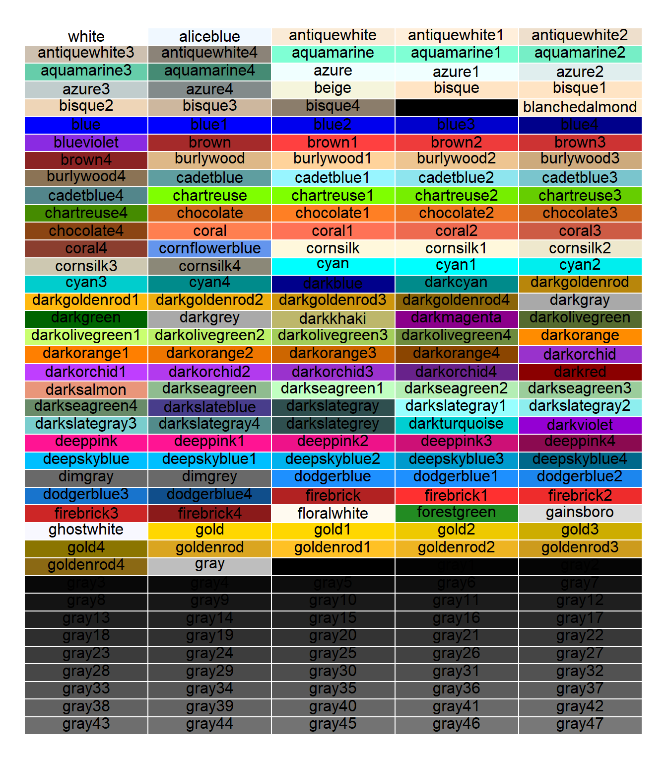
Figure 7.7: Names and appearance of the first 200 colors in R
7.3 Points and Lines
The default point is a filled circle. We showed how to use the shape = parameter in the geom_point function to specify a different shape in Chapter 1. We have also shown how to map shapes to the levels of a categorical variable in the aes function in Chapters 1 and 4.
The default line type is a solid line. In Figure 7.8 we replicate Figure 7.5 using the linetype parameter in the geom_line function. We visualize the results for state = "Melaka".
mysdeaths %>%
  filter(date >= as.Date("2021-02-24")) %>%
  select(date, state, deaths_new_dod, deaths_pvax, deaths_fvax) %>%
  filter(state == "Melaka") %>%
  gather(key = "death_type", value = "deaths", 3:5) %>%
  mutate(death_type = case_when(
    death_type == "deaths_new_dod" ~ "1. New deaths",
    death_type == "deaths_pvax" ~ "2. Partial vax",
    death_type == "deaths_fvax" ~ "3. Full vax",
    TRUE ~ NA_character_)) %>%
  ggplot(aes(x = as.Date(date),
             y = deaths,
             linetype = death_type,
             color = death_type)) +
  geom_line() +
  scale_y_continuous(breaks = seq(0, 20, 5),
                     limits = c(0, 20)) +
  scale_x_date(date_breaks = "1 month",
               date_labels = "%b-%Y") +
  labs(title = "Melaka Covid Deaths by Category",
       subtitle = "Since 24 Feb 2021",
       x = "Date",
       y = "Deaths",
       linetype = "Death Category",
       color = NULL)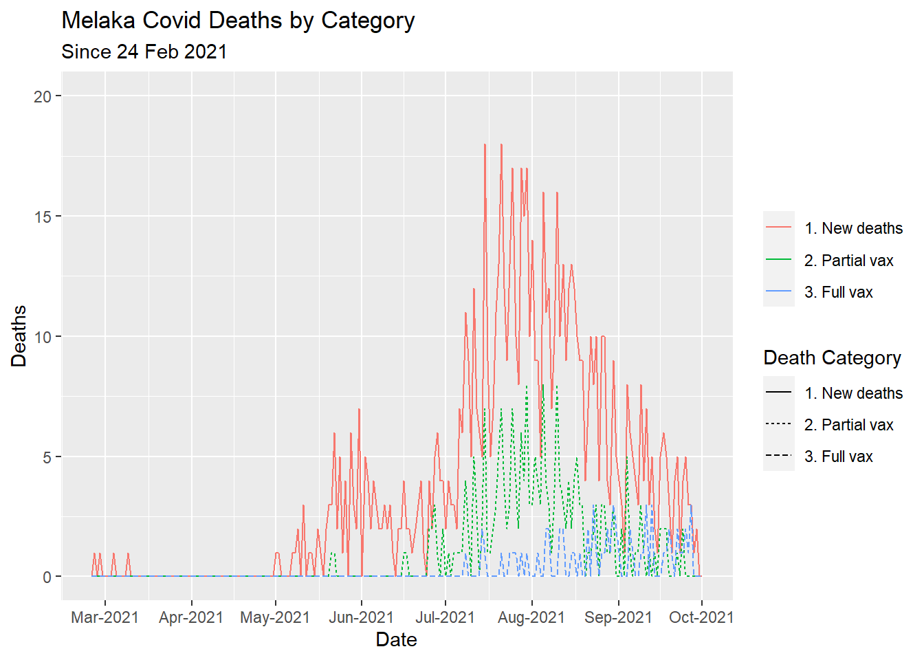
Figure 7.8: Types of Covid deaths for selected state
7.4 Legends
Legends are automatically created when variables or columns are mapped to parameters like color, fill, linetype, shape, size, or alpha. We have seen how this can be customized using the theme and/or the labs function.
We replicate Figure 7.8 for state == "Johor". We change the default legend.position position on the right and place it at the bottom with
theme(legend.position = "left"). We also set the alignment of the legend title using the theme(legend.title.align = 0.5) (0=left, 0.5=center, 1=right).
mysdeaths %>%
  filter(date >= as.Date("2021-02-24")) %>%
  select(date, state, deaths_new_dod, deaths_pvax, deaths_fvax) %>%
  filter(state == "Johor") %>%
  gather(key = "death_type", value = "deaths", 3:5) %>%
  mutate(death_type = case_when(
    death_type == "deaths_new_dod" ~ "1. New deaths",
    death_type == "deaths_pvax" ~ "2. Partial vax",
    death_type == "deaths_fvax" ~ "3. Full vax",
    TRUE ~ NA_character_)) %>%
  ggplot(aes(x = as.Date(date),
             y = deaths,
             color = death_type)) +
  geom_line() +
  scale_y_continuous(breaks = seq(0, 60, 5),
                     limits = c(0, 60)) +
  scale_x_date(date_breaks = "1 month",
               date_labels = "%b-%Y") +
  labs(title = "Johor Covid Deaths by Category",
       subtitle = "Since 24 Feb 2021",
       x = "Date",
       y = "Deaths",
       color = "Death Category") +
  theme(legend.position = "left") +
  theme(legend.title.align = 0.5)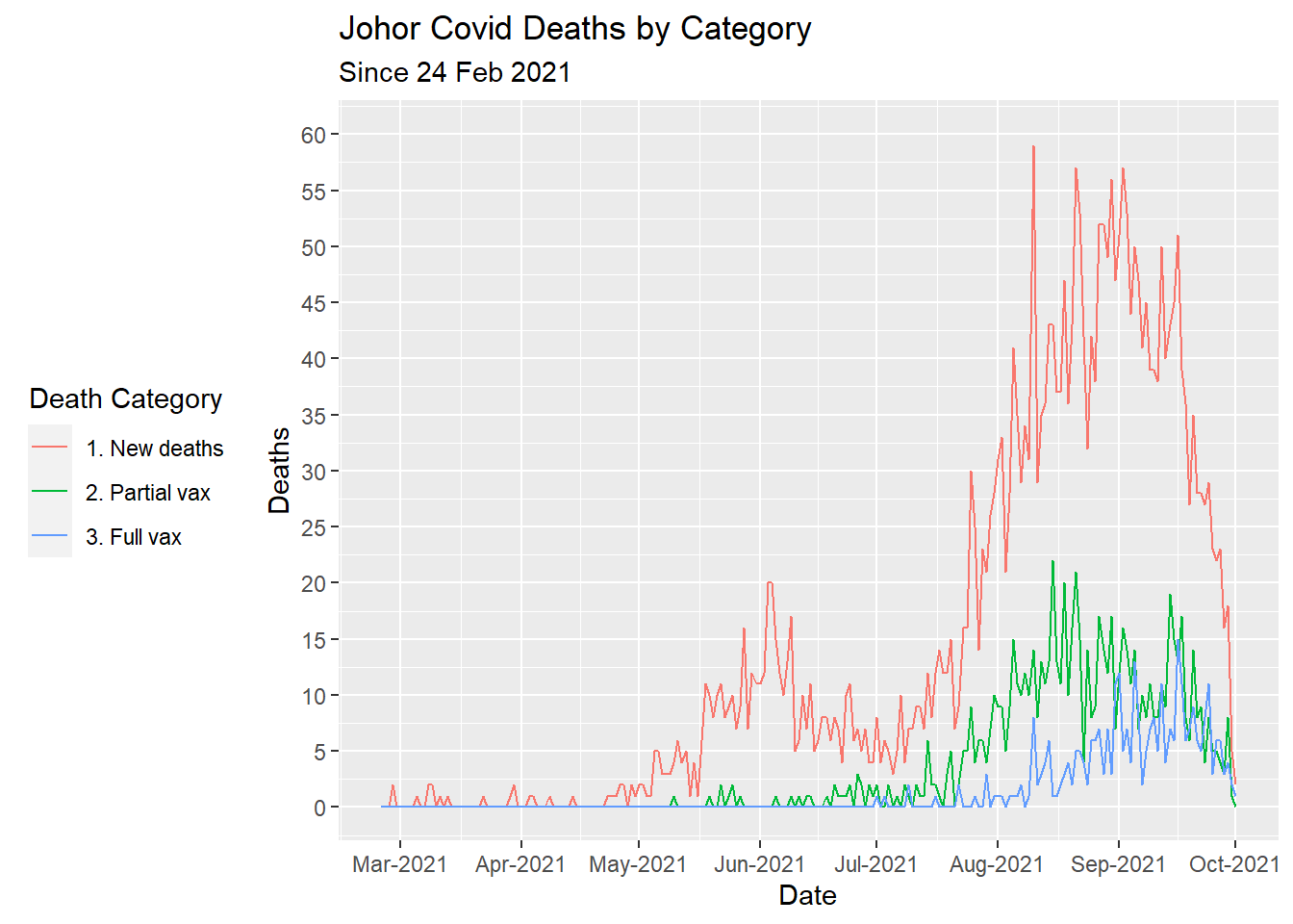
Figure 7.9: Types of Covid deaths for selected state
7.5 Annotations
Visualizing data through the basic graph elements like points, lines and bars can always be augmented by other information that can help the viewer interpret the data. We can also add individual pictures, emojis, or text elements to add extra contextual information, highlight an area of the plot, or add some descriptive text about the data.22
We will apply some of these in the coming chapters.
7.6 Discussion
Customizing the appearance of graphs can be overdone. We prefer to keep it simple and minimal. We have covered the common options with some examples on our actual Covid deaths data. Perhaps it is better to look at the other options when we need them in later chapters of the book.
References
https://github.com/MoH-Malaysia/covid19-public/blob/main/epidemic/deaths_state.csv↩︎
https://www.linkedin.com/posts/azman-hussin-00573248_gametheory-covid-activity-6847747068031840256-QubM↩︎
https://www.bloomberg.com/news/articles/2021-02-24/malaysia-starts-coronavirus-vaccination-pm-gets-first-shot↩︎