Chapter 18 Regession Assumptions
18.1 Get Started
This chapter explores a set of regression assumptions in the context of the life expectancy regression model developed in Chapter 17. To follow along in R, make sure to load the countries2 data set, as well as the libraries for the following packages: DescTools, lmtest, sandwich, and stargazer.
18.2 Regression Assumptions
The level of confidence we can have in regression estimates (slopes and significance levels) depends upon the extent to which certain assumptions are met. These assumptions are outlined briefly below and applied to the life expectancy model, using diagnostic tests when necessary. Several of these assumptions have to do with characteristics of the error term in the population (\(\epsilon_i\)), which, of course, we cannot observe, so we evaluate them using the sample residuals (\(e_i\)) instead. Some of these assumptions have been discussed in some detail in earlier chapters, while others have not.
18.3 Linearity
The pattern of the relationship between x and y is linear; that is, the rate of change in y for a given change in x is constant across all values of x, and the model for a straight line fits the data best. The example of the curvilinear relationship between doctors per 10,000 and life expectancy shown in Chapter 17 is a perfect illustration of the problem that occurs when a linear model is applied to a non-linear relationship: the straight line is not the best fitting line and the model will fall short of producing the least squared error possible for a given set of variables. The best way to get a sense of whether you should test a curvilinear model to examine the bi-variate relationships using scatterplots. This is how we sniffed out the curvilinear relationship for docs10k in Chapter 17. The scatterplots for the relationships between life expectancy and all five of the original independent variables are presented in Figure 18.1.
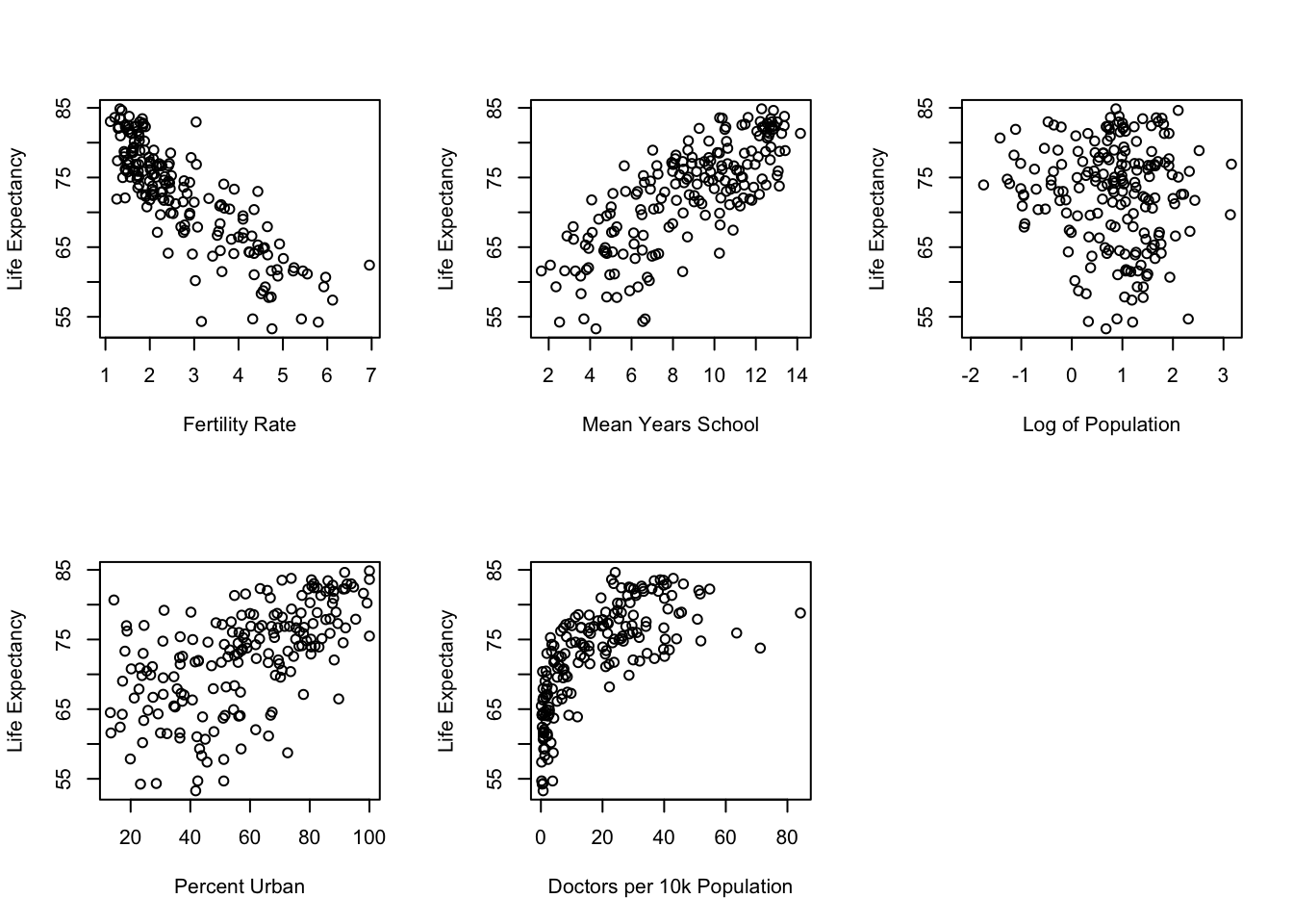
Figure 18.1: Scatterplots Can be Used to Evaluate Linearity
Based on a visual inspection of these scatterplots, docs10k is the only variable that appears to violate the linearity assumption. Since this was addressed by using the log (base 10) of its values, no other changes in the model appear to be necessary, at least due to non-linearity.
18.5 No Perfect Multicollinearity
The assumption is that, for multiple regression, none of the independent variables is a perfect linear combination of the others. At some level, this is a non-issue when analyzing data, as R and other programs will automatically drop a variable from the model if it is perfectly collinear with one or more other variables. Still, we know from the discussion in Chapter 17 that there is almost always some level of collinearity in a multiple regression model and it can create problems if the level is very high. We know from Chapter 17 that the problem with collinearity is that it inflates the slope standard errors, resulting in suppressed t-scores and p-values. Because we have added food_def to the model since the initial round of collinearity testing in Chapter 17, we should take a look at the VIF statistics for the final model.
#Check VIF statistics for new model
VIF(fit2)
countries2$fert1520 countries2$mnschool log10(countries2$pop19_M)
3.63 3.84 1.08
countries2$urban log10(countries2$docs10k) countries2$food_def
1.84 5.18 1.59 Still no major problem with collinearity. As mentioned in Chapter 17, there is no universally accept cutoff point for what constitutes too-high collinearity. One thing to keep in mind is that the impact of collinearity on levels of statistical significance is more acute for small rather than large samples. This is because as the sample size increases, standard errors decrease and t-scores increase (Chapter 8). As a result, even though collinearity still leads to decreased t-scores in large samples, there is a smaller chance that the reduced size of the t-score will affect the hypothesis testing decision, compared to small samples.
18.6 The Mean of the Error Term equals zero
If the expected (average) value of the error term does not equal zero, then it is likely that the constant is biased. This is easy enough to test using the sample residuals:
#Get the mean prediction error
mean(residuals(fit2), na.rm=T)
[1] 2.81e-17The mean error in the regression model is .0000000000000000281, pretty darn close to 0.
If you find that the mean of the error term is different from zero, it could be due to specification error, so you should look again at whether you need to transform any of your existing variables or incorporate other variables into the model.
18.7 The Error Term is Normally Distributed
This assumption is important to having confidence in estimates of statistical significance. In practice, when working with a large sample, researchers tend not to worry much about the normality of the error term unless the deviation from normality is quite severe. There are a number of different ways to check on this, including plotting the residuals in a histogram to see if they appear to be normally distributed:
#Get histogram of stored residuals from fit2
hist(residuals(fit2), prob=T, ylim=c(0, .12) )
#save the mean and standard deviation of residuals
m<-mean(residuals(fit2), na.rm=T)
std<-sd(residuals(fit2), na.rm=T)
#Create normal curve using the mean and standard deviation
curve(dnorm(x,mean=m,sd=std), add=T)
#Add legend
legend("topright", legend=c("Normal Curve"), lty=1, cex=.7)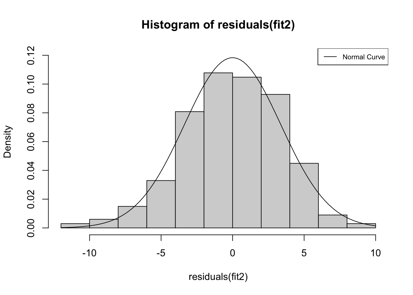
The contours of this histogram appear to be approaching a normal distribution, but it is hard to tell if the pattern is similar enough to normally distributed that we can be confident that we are not violating the normality assumption. Instead, we can use the Shapiro-Wilk normality test to test the null hypothesis that the residuals from this model are normally distributed. If the p-value generated from this test is less than .05, then we reject the null hypothesis and conclude that the residuals are not normally distributed. The results of this test (shapiro.test) are presented below.
#Test for normality of fit2 residuals
shapiro.test(residuals(fit2))
    Shapiro-Wilk normality test

data:  residuals(fit2)
W = 1, p-value = 0.3
The p-value is greater than .05, so we can conclude that the distribution of residuals from this model do not deviate significantly from a normal distribution.
If the distribution of the error term does deviate significantly from normal, it could be the result of outliers or specification error (e.g., omitted variable or non-linear relationship).
18.8 Constant Error Variance (Homoscedasticity)
The variance in prediction error (residuals) is the same across all values of the independent variables. In other words if you predict y with x, it is expected that the amount of prediction error (spread of data points around the regression line) should be roughly the same as you move from low to high values of x, that x does not do a better job predicting y in some ranges of x than in others. This assumption is important because the estimates of statistical significance are based on the amount of error in prediction. If that error varies significantly across observations (heteroscedasticity), then we might be over or underestimating statistical significance. Importantly, violating this assumption does not mean that the regression slopes are biased, just that the reported standard errors of the slopes, and, hence, t-scores are likely to be incorrect.
A simple way to evaluate homoscedasticity is to exam a scatterplot of the model residuals across the range of predicted outcomes, looking for evidence of substantial differences in the spread of the residuals over the range of outcomes. The classic pattern for a violation of this assumption is a cone-like pattern in the residuals, with a narrow range of error at one end and a wider range at the other. The graph below exams this assumption for life expectancy model.
#Plot residuals from model as a function of predicted values
plot(predict(fit2), residuals(fit2))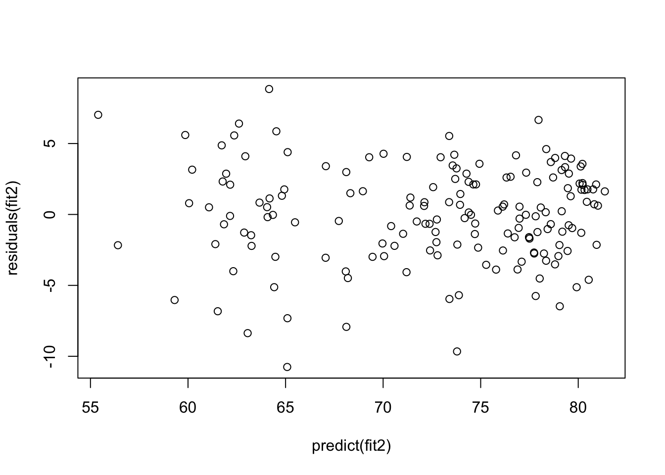
Though the pattern is not striking, it looks like there is a tendency for greater variation in error at the low end of the predicted outcomes than at the high end, but it is hard to tell if this is a problem based on simply eyeballing the data. Instead, we can test the null hypotheses that variance in error is constant, using the Breusch-Pagan test (bptest) from the lmtest package:
bptest(fit2)
    studentized Breusch-Pagan test

data:  fit2
BP = 20, df = 6, p-value = 0.002
With a p-value of .002, we reject the null hypothesis that there is constant variance in the error term. So, what to do about this violation of the homoscedasticity assumption? Most of the solutions, including those discussed below, are a bit beyond the scope of an introductory textbook. Nevertheless, I’ll illustrate a set of commands that can be used to address this issue.
There are a number of ways to address heteroscedasticity, mostly by weighting the observations based on the size of their error. This approach, called Weighted Least Squares, entails determining if a particular variable (x) is the source of the heteroscedasticity and then weight the observations by the reciprocal of that variable (\(1/x\)), or to transform the residuals and weight the data by the reciprocal of that transformation. Alternatively, you can use the vcovHC function, which adjusts the standard error estimates so they account for the non-constant variance in the error. Then, we can incorporate information created by vcovHC into the stargazer command to produce a table with new standard errors, t-scores, and p-values. The code below shows how to do this.50
#Use the regression model (fit2) and method HC1 in 'vcovHC' function.
#Store the new covariance matrix in object "hc1"
hc1<-vcovHC(fit2, type="HC1")
#Save the new "Robust" standard errors in a new object
robust.se <- sqrt(diag(hc1))
#Integrate the new standard error into the regression output
#using stargazer.  Note that the model (fit2) is listed twice, so a
#comparison can be made. To only show the corrected model, only list fit2
#once, and change "se=list(NULL, robust.se)" to "se=list(robust.se)"
stargazer(fit2, fit2, type = "text",se=list(NULL, robust.se),
          column.labels=c("Original", "Corrected"),
          dep.var.labels=c("Life Expectancy"),
          covariate.labels = c("Fertility Rate",
                               "Mean Years of Education",
                               "Log10 Population", "% Urban",
                               "Log10 Doctors/10k",
                               "Food Deficit"))
===========================================================
                                   Dependent variable:
                               ----------------------------
                                     Life Expectancy
                                  Original      Corrected
                                    (1)            (2)
-----------------------------------------------------------
Fertility Rate                   -2.680***      -2.680***
                                  (0.409)        (0.492)

Mean Years of Education            0.232          0.232
                                  (0.167)        (0.163)

Log10 Population                   -0.281        -0.281
                                  (0.341)        (0.339)

% Urban                            0.028*        0.028*
                                  (0.016)        (0.016)

Log10 Doctors/10k                 2.390**        2.390*
                                  (0.968)        (1.250)

Food Deficit                      0.093***      0.093***
                                  (0.021)        (0.020)

Constant                         63.100***      63.100***
                                  (2.950)        (3.450)

-----------------------------------------------------------
Observations                        167            167
R2                                 0.790          0.790
Adjusted R2                        0.782          0.782
Residual Std. Error (df = 160)     3.430          3.430
F Statistic (df = 6; 160)        100.000***    100.000***
===========================================================
Note:                           *p<0.1; **p<0.05; ***p<0.01
Two important things to note about these new estimates. First, as expected, the standard errors changed for virtually all variables. Most of the changes were quite small and had little impact on the p-values. The most substantial change occurred for docs10k, whose slope is still statistically significant using a one-tailed test. The other thing to note is that this transformation had no impact on the slope estimates, reinforcing the fact that heteroscedasticity does not lead to biased slopes but does render standard errors unreliable.
18.9 Independent Errors
The errors produced by different values of the independent variables are unrelated to each other; that is, the errors from one observation do not affect the errors of other observations. This is often referred to as serial correlation and is often a problem for time-series data, which we have not worked with much at all in this book. Some academic areas, such as economics and certain sub-fields of political science, rely heavily on time series data, and scholars in those areas need to be examine their models closely in search of serial correlation. When serial correlation is present, it leads to suppressed standard errors, which creates inflated t-scores, and can lead researchers to falsely conclude that some relationships are statistically significant when they are not.
18.10 Next Steps
You’ve made it through the book! Give yourself a pat on the back. You’ve covered a lot of material and you’ve probably done so during a single semester while taking other courses. Just think back to the beginning of the book when you were first learning about a programming language called R and just dipping your toe into data analysis with simple frequency tables. Those were important things to learn, but you’ve picked up a lot more since then.
There is no “Next Step” from here in this book, but there are some things you can do to build on what you learned. First and foremost, don’t let what you’ve learned sit on the shelf very long. It’s not like there is an expiration date on what you’ve learned, but it will start to fade and be less useful if you don’t find ways to use it. The most obvious thing you can do is follow up with another course. One type of course that would be particularly useful is one that focuses primarily on regression analysis and its extensions. While the last four chapters in this book focused on regression analysis, they really just scratched the surface. Taking a stand-alone course on regression analysis will reinforce what you’ve learned and provide you with a stronger base and a deeper understanding of this important method. Be careful, though, to make sure you find a course that is pitched at the right level for you. For instance, if you felt a bit stretched by some of the technical aspects of this book, you should not jump right into a regression course offered in the math or statistics department. Instead, a regression-based course in the social sciences might be more appropriate for you. But if you are comfortable with a more math-stats orientation, then by all means find a regression course in the math or statistics department at your school.
There are other potentially fruitful follow-up courses you might consider. If you were particularly taken with the parts of this book that focused on survey analysis using the 2020 ANES data, you should look for a course on survey research. These courses are usually found in political science, sociology, or mass communications departments. At the same time, if you found the couple of very brief discussions of experimental research interesting, you could follow up with a course on analyzing experimental data. The natural sciences are a “natural”51 place to find these courses, but if your tastes run more to the social sciences, you should check out the psychology department on your campus for these courses.
Since you’ve already invested some valuable time learning how to use R, you should also find ways to build on that part of the course. If you take another data analysis course, try to find one that uses R so you can continue to improve your programming skills. This brings me to one of the most important things you should look for in other data analysis courses: make sure the course requires students to do “hands-on” data analysis problems utilizing real-world data. It would be great if the course also required the use of R, but one of the most important things is that students are required to use some type of data analysis program (e.g., R, SPSS, Stata, Minitab, Excel, etc.) to do independent data analysis. Absent this, you might learn about data analysis, but you will not learn to do data analysis.
18.11 Exercises
18.11.1 Concepts and Calculations
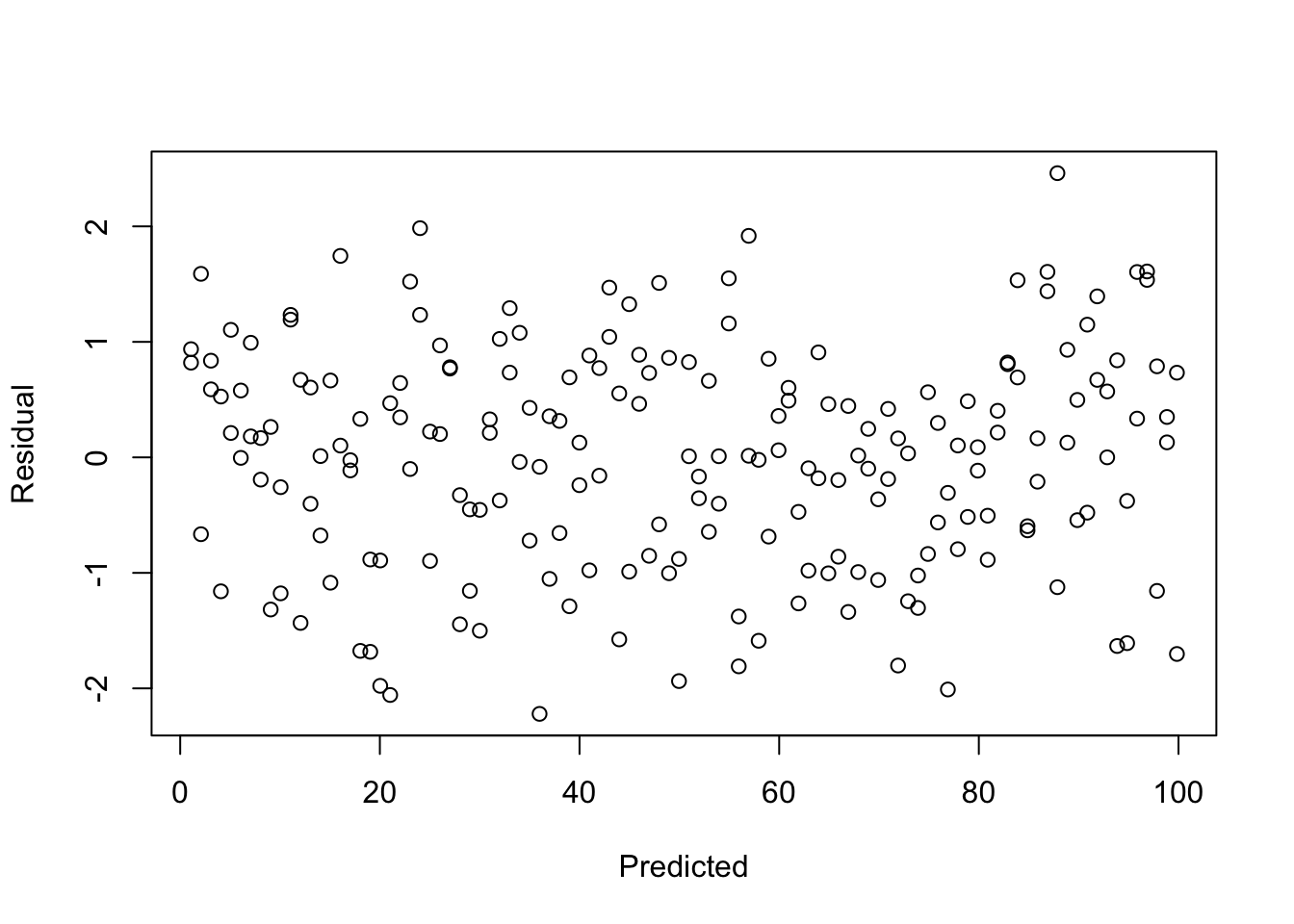
- Do any regression assumptions appear to be violated in this scatterplot? If so, which one? Explain your answer. If you think an assumption was violated, discuss what statistical test you would use to confirm your suspicion.
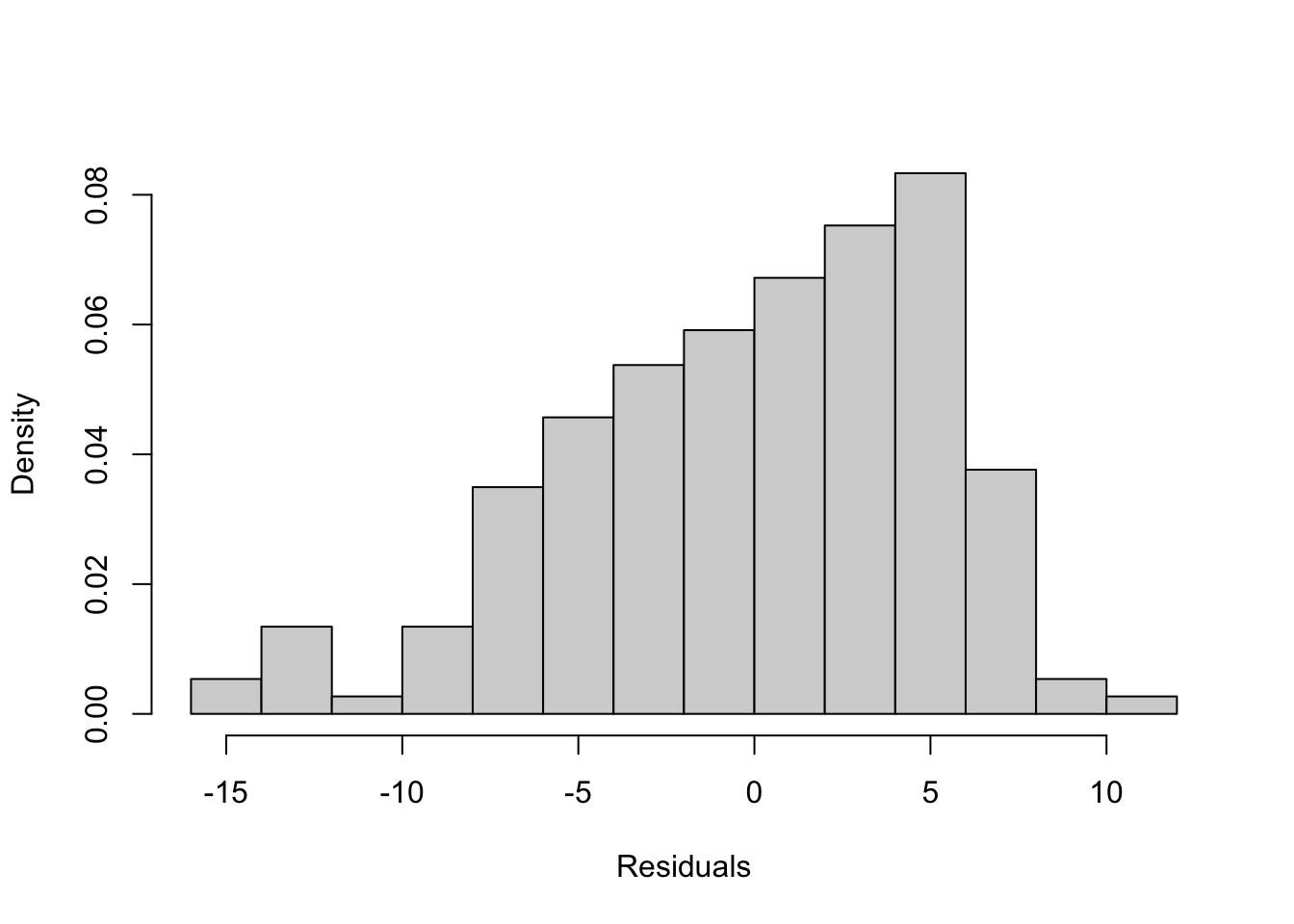
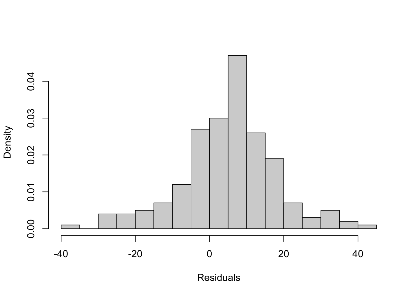
- Do any regression assumptions appear to be violated in this histogram? If so, which one? Explain your answer. If you think an assumption was violated, discuss what statistical test would you use to confirm your suspicion.
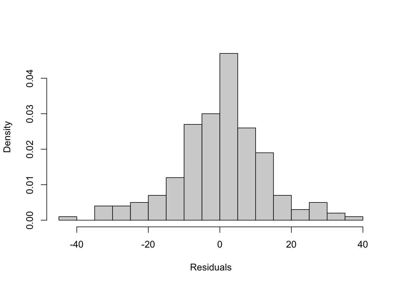
- Do any regression assumptions appear to be violated in this histogram? If so, which one? Explain your answer. If you think an assumption was violated, discuss what statistical test you would use to confirm your suspicion.
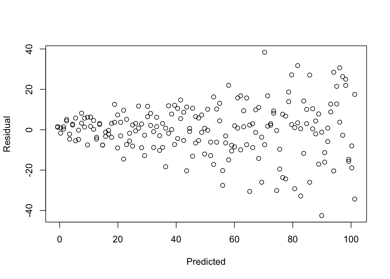
- Do any regression assumptions appear to be violated in this scatterplot? If so, which one? Explain your answer. If you think an assumption was violated, discuss what statistical test you would use to confirm your suspicion.
- Do any regression assumptions appear to be violated in this histogram? If so, which one? Explain your answer. If you think an assumption was violated, discuss what statistical test you would use to confirm your suspicion.
18.11.2 R Problems
These problems focus on the same regression model used for the R exercises in Chapter 17. With the states20 data set, run a multiple regression model with infant mortality (infant_mort) as the dependent variable and per capita income (PCincome2020), the teen birth rate (teenbirth), percent of low birth weight births (lowbirthwt), southern region (south), and percent of adults with diabetes (diabetes) as the independent variables.
Use a scatterplot matrix to explore the possibility that one of the independent variables violates the linearity assumption. If it looks like there might be a violation, what should you do about it?
Test the assumption that the mean of the error term equals zero.
Use both a histogram and the
shapiro.testfunction to test the assumption that the error term is normally distributed.Plot the residuals from the infant mortality model against the predicted values and evaluate the extent to which the assumption of constant variation in the error term is violated. Use the
bptestfunction as a more formal test of this assumption. Interpret both the scatterplot and the results of thebptest.The infant mortality model includes five independent variables. While parsimony is a virtue, it also creates the potential for omitted variable bias. Look at the other variables in the
states20data set and identify one of them that you think might be an important influence on infant mortality and whose exclusion from the model might bias the estimated effects of the other variables. Justify your choice. Add the new variable to the model, usestargazerto display the new model alongside the original model, and discuss the differences between the models and whether the original estimates were biased.
