Chapter 9 Hypothesis Testing

Getting Started

In this chapter, the concepts used in Chapters 7 & 8 are extended to focus more squarely on making statistical hypothesis testing. The focus here is on taking the abstract ideas that are the foundation for hypothesis testing and applying them to some concrete examples. The only thing you need to load in order to follow among is the anes20.rda data set.

The Logic of Hypothesis Testing

When engaged in the process of hypothesis testing, we are essentially asking “what is the probability that the statistic found in the sample could have come from a population in which it is equal to some other, specified, value?” As discussed in Chapter 8, social scientists want to know something about a population value but frequently are only able to work with sample data. We generally think the sample data represent the population fairly well but we know that there will be some sampling error. In Chapter 8, we took this into account using confidence intervals around sample statistics. In this chapter, we apply some of the same logic to determine if the sample statistic is different enough from a hypothesized population parameter that we can be confident it did not occur just due to sampling error. (Come back and reread this paragraph when you are done with this chapter; it will make a lot more sense then).

We generally consider two different types of hypotheses, the null and alternative (or research) hypotheses.

Null Hypothesis (H₀): This hypothesis is tested directly. It usually states that the population parameter ($\mu$) is equal to some specific value, even if the sample statistic ($\bar{x}$) is a different value. The implication is that the difference between the sample statistic and the hypothesized population parameter is attributable to sampling error, not a real difference. We usually hope to reject the null hypothesis. This might sound strange now, but it will make more sense to you soon.
Alternative (research) Hypothesis (H₁): This is a substantive hypothesis that we think is true. Usually, the alternative hypothesis posits that the population parameter does not equal the value specified in H₀. We don’t actually test this hypothesis directly. Rather, we try to build a case for it by showing that the sample statistic is different enough from the population value hypothesized in H₀ that it is unlikely that the null hypothesis is correct.

We can use what we know about the z-distribution to test the validity of the null hypothesis by stating and testing hypotheses about specific values of population parameters. Consider the following problem:

A data analyst in the Human Resources department for a large metropolitan county is asked to evaluate the impact of a new method of documenting sick leave among county employees. The new policy is intended to cut down on the number of sick leave hours taken by workers. Last year, the average number of hours of sick leave taken by workers was 59.2 (about 7.4 days), a level determined to be too high. To evaluate if the new policy is working, the analyst took a sample of 100 workers at the end of one year under the new rules and found a sample mean of 54.8 hours (about 6.8 days), and a standard deviation of 15.38. The question is, does this sample mean represent a real change in sick leave use, or does it only reflect sampling error? To answer this, we need to determine how likely it is to get a sample mean of 54.8 from a population in which $\mu=59.2$.

Using Confidence Intervals

As alluded to at the end of Chapter 8, you already know one way to test hypotheses about population parameters by using confidence intervals. In this case, the county data analyst can calculate the lower- and upper-limits of a 95% confidence interval around the sample mean (54.8) to see if it includes $\mu$ (59.2):

\[c.i._{.95}=54.8\pm {1.96(S_{\bar{x}})}\] \[S_{\bar{x}}=\frac{15.38}{\sqrt{100}}=1.538\] \[c.i._{.95}=54.8 \pm 1.96(1.538)\] \[c.i._{.95}=54.8 \pm 3.01\] \[51.78\le \mu \le57.81\]

From this sample of 100 employees, after one year of the new policy in place, the county analyst is able to estimate that there is a 95% chance that the interval between 51.78 and 57.81 includes $\mu$, and the probability that $\mu$ is outside this range is less than .05. Based on this alone we can say there is less than a 5% chance that the number of hours of sick leave taken is the same that it was in the previous year. In other words, there is a fairly high probability that fewer sick leave hours were used in the year after that policy change than in the previous year.

Direct Hypothesis Tests

We can be a bit more direct and precise by setting this up as a hypothesis test and then calculating the probability that the sample mean came from a population in which the null hypothesis is true. First, the null hypothesis.

\[H_{0}:\mu=59.2\]

This is saying is that there is no real difference between last year’s mean number of sick days ($\mu$) and the sample we’ve drawn from this year ($\bar{x}$). Even though the sample mean looks different from 59.2, the true population mean is 59.2, and the sample statistic is just a result of random sampling error. After all, if the population mean is equal to 59.2, any sample drawn from that population will produce a mean that is different from 59.2, due to sampling error. In other words, H₀, is saying that the new policy had no effect, even though the sample mean suggests otherwise.

Because the county analyst is interested in whether the new policy reduced the use of sick leave hours, the alternative hypothesis is:

\[H_{1}:\mu < 59.2\]

Here, we are saying that the sample statistic is different enough from the hypothesized population value (59.2) that it is unlikely to be the result of random chance; that represents real change, and the population value is less than 59.2.

Note here that we are not testing whether the number of sick days is equal to 54.8 (the sample mean). Instead, we are testing whether the average hours of sick leave taken this year is lower than the average number of sick days taken last year. The alternative hypothesis reflects what we really think is happening; it is what we’re really interested in. We test the null hypothesis as a way of gathering evidence to support the alternative.

Sampling Distributions and Hypothesis Testing

To answer to test the null hypothesis we need to ask how likely it is that a sample mean of this magnitude (54.8) could be drawn from a population in which $\mu\text{= 59.2}$. We know that we would get lots of different mean outcomes if we took repeated samples from this population. We also know that most of them would be clustered near $\mu$ and a few would be relatively far away from $\mu$ at both ends of the distribution. All we have to do is estimate the probability of getting a sample mean of 54.8 from a population in which $\mu\text{= 59.2}$. If the probability of drawing $\bar{x}$ from $\mu$ is small enough, then we can reject H₀.

We can assess this probability by converting the difference between $\bar{x}$ and $\mu$ into a z-score, and then use what we know about sampling distributions to calculate the probability of getting $\bar{x}$ from a population in which the null hypothesis is true (see Figure 9.1).

[Figure************************ 9.1 ************************about here]

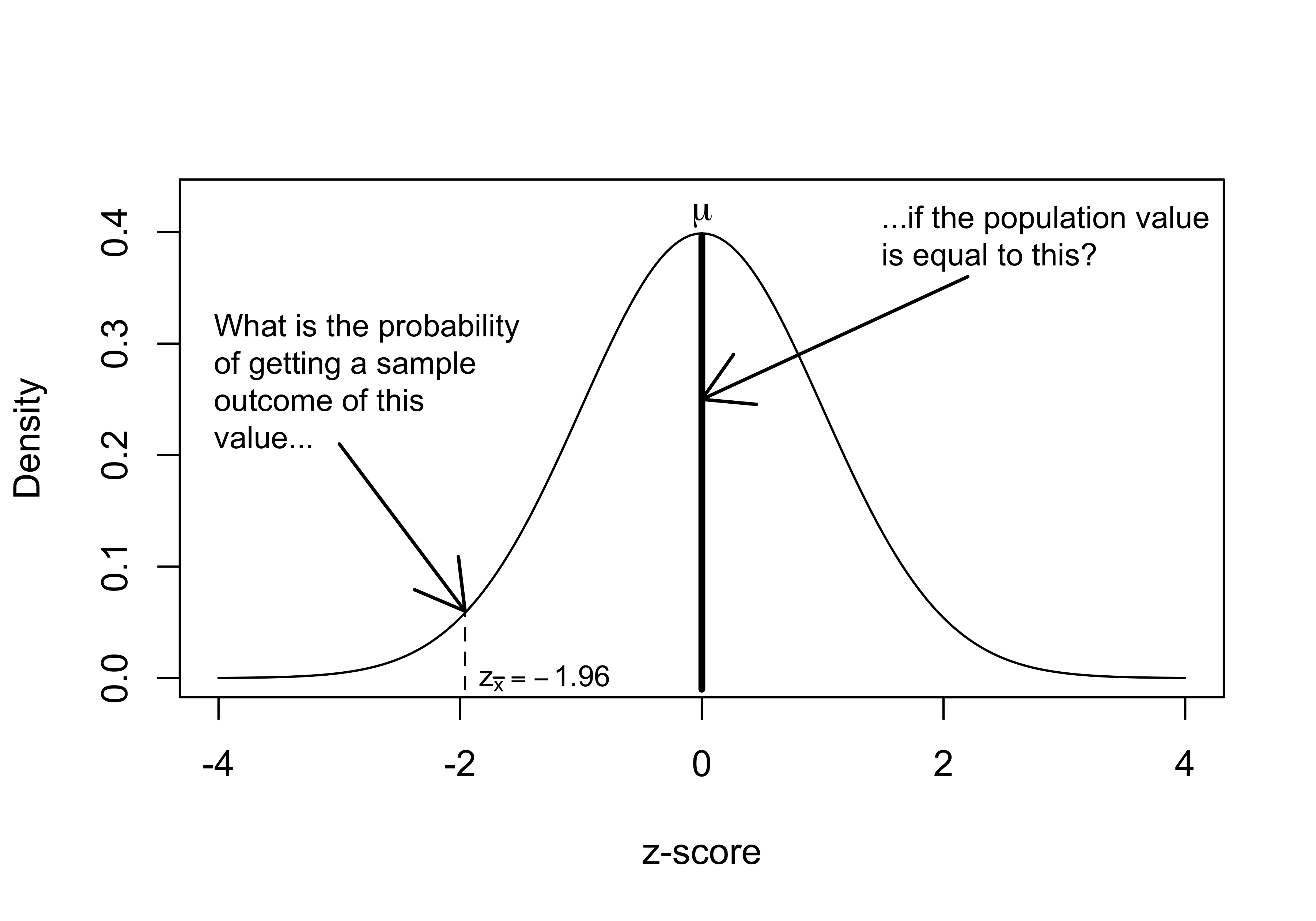
Figure 9.1: The Logic of Hypothesis Testing

The essential question in hypothesis testing is, “What is the probability of getting a particular sample outcome ( $\bar{x}$ ) from a population in which population value is equal to something else ($\mu$)?” The process for answering that question in laid out in Figure 9.1, which illustrates a sampling distribution in which the z-score for a sample mean ($\bar{x}$) is -1.96. We can calculate the probability of getting a sample mean of this magnitude or lower (z=-1.96) by estimating the area under the curve to the left of -1.96. The area on the tail of the distribution used for hypothesis testing is referred to as the $\alpha$ (alpha) area. As shown below, the alpha area for z=-1.96 is .025. This result is also commonly referred to as the p-value, for probability value.

pnorm(-1.96)

[1] 0.0249979

With this information, we can say that the probability of drawing a sample mean with a z-score less than or equal to -1.96 from a population in which the null hypothesis is true ($\mu=0$, in this case) is about .025. This can also be interpreted as saying that probability that the observed sample outcome occurred by chance is about .025. This is pretty low, so we reject the null hypothesis. The smaller the p-value, the more confident you can be in rejecting the null hypothesis.

To reiterate from above, the critical step in moving from empirical data to hypothesis testing is to convert your sample statistic to a z-score. Once you’ve done that, you simply use what you know about sampling distributions to test the null hypothesis.

Critical Values. A common and fairly quick way to use the z-score in hypothesis testing is by comparing it to the critical value (c.v.) for z. The critical value is the z-score associated with the probability level (p-value) required to reject the null hypothesis. To determine the critical value of z, we need to determine what the probability threshold is for rejecting the null hypothesis. In other words, how confident do you have to be that the observed sample outcome did not come from a population in which the null hypothesis is true before you can reject the null hypothesis? In the social sciences it is fairly standard to consider any probability level lower than .05 sufficient for rejecting the null hypothesis. This probability level is also known as the significance level.

Typically, the critical value is the z-score that gives us .05 as the area on the tail (left in this case) of the normal distribution. Looking at the z-score table from Chapter 6, or using the qnorm function in R, we see that this is z = -1.645. The area beyond the critical value is referred to as the critical region, and is sometimes also called the area of rejection: if the z-score falls in this region, the null hypothesis is rejected.

#Get the z-score for .05 area at the lower tail of the distribution
qnorm(.05, lower.tail = T)

[1] -1.644854

Once we have the $c.v.$, we can calculate the z-score for the difference between $\bar{x}$ and $\mu$. The z-score will be positive if $\bar{x}-\mu >0$ and negative if $\bar{x}-\mu <0$. If $|z| > |z_{cv}|$, then we reject the null hypothesis:

So let’s get back to the sick leave example.

First, what’s the critical value? -1.65 (make sure you understand why this is the value)
What is the obtained value of z?

\[z=\frac{\bar{x}-\mu}{S_{\bar{x}}} = \frac{54.8-59.2}{1.538} = \frac{-4.4}{1.538}= -2.86\]

This z-score of -2.86 means that the sample mean (54.8) is 2.86 standard errors lower the hypothesize population value (59.2).

If the |z| is greater than the |c.v.|, then reject H₀. If the |z| is less than the critical value, then fail to reject H₀

In this case z (-2.86) is of much greater (absolute) magnitude than c.v. (-1.65), so we reject the null hypothesis and conclude that $\mu$ is probably less than 59.2. By rejecting the null hypothesis we build a case for the alternative hypothesis, though we never test the alternative directly. Rejecting the null hypothesis means that we are saying that the difference is statistically significant, representing a real difference rather than random error.

We can be a bit more precise about the level of confidence in rejecting the null hypothesis (the level of statistical significance) by estimating the alpha area to the left of z=-2.86:

#Area under to curve to the left of -2.86
pnorm(-2.86)

[1] 0.002118205

This alpha area (or p-value) is close to zero, reinforcing the conclusion that we can confidently reject the null hypothesis. Check out Figure 9.2 as an illustration of how unlikely it is to get a sample mean of 54.8 (thick solid line) from a population in which $\mu=59.2$, (thin solid line) based on our sample statistics. Remember, the area to the left of the critical value (dashed line) is the critical region, equal to .05 of the area under the curve, and the sample mean is far to the left of this point.

One useful way to think about this p-value (and others like it) is that if we took 1000 samples of 100 workers from a population in which $\mu=59.2$, and calculated the mean hours of sick leave taken for each sample, only two samples would give you a result equal to or less than 54.8 simply due to sampling error. In other words, there is a 2/1000 chance that the sample mean was the result of random variation instead of representing a real difference from the hypothesized value.

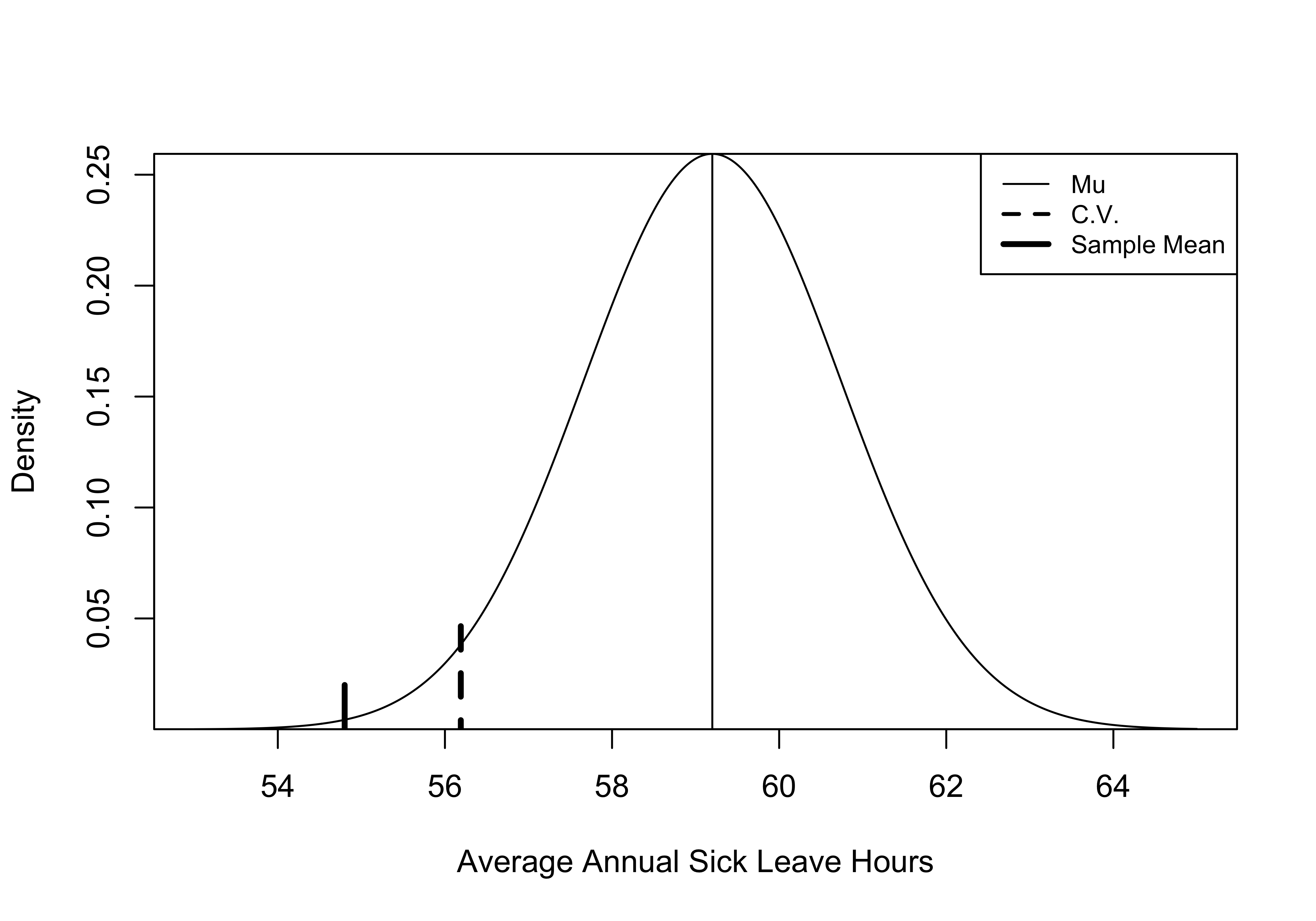
Figure 9.2: An Illustration of Key Concepts in Hypothesis Testing

[Figure******************** 9.2 ********************about here]

One-tail or Two?

Note that we were explicitly testing a one-tailed hypothesis in the example above. We were saying that we expect a decrease in the number of sick days used, due to the new policy. But suppose someone wanted to argue that there was a loophole in the new policy that might make it easier for people to take sick days. These sorts of unintended consequences almost always occur with new policies. Given that it could go either way ($\mu$ could be higher or lower than 59.2), the county data analyst who is evaluating this policy might decide to test a two-tailed hypothesis: that the new policy could create a difference in sick day use, and that difference could be positive, or it could be negative.

$H_{1}:\mu \ne 59.2$

The process for testing two-tailed hypotheses is exactly the same, except that we use a larger critical value because even though the $\alpha$ area is the same (.05), we must now split it between two tails of the distribution. Again, this is because we are not sure if the policy will increase or decrease sick leave. When the alternative hypothesis does not specify a direction, the two-tailed test is most appropriate.

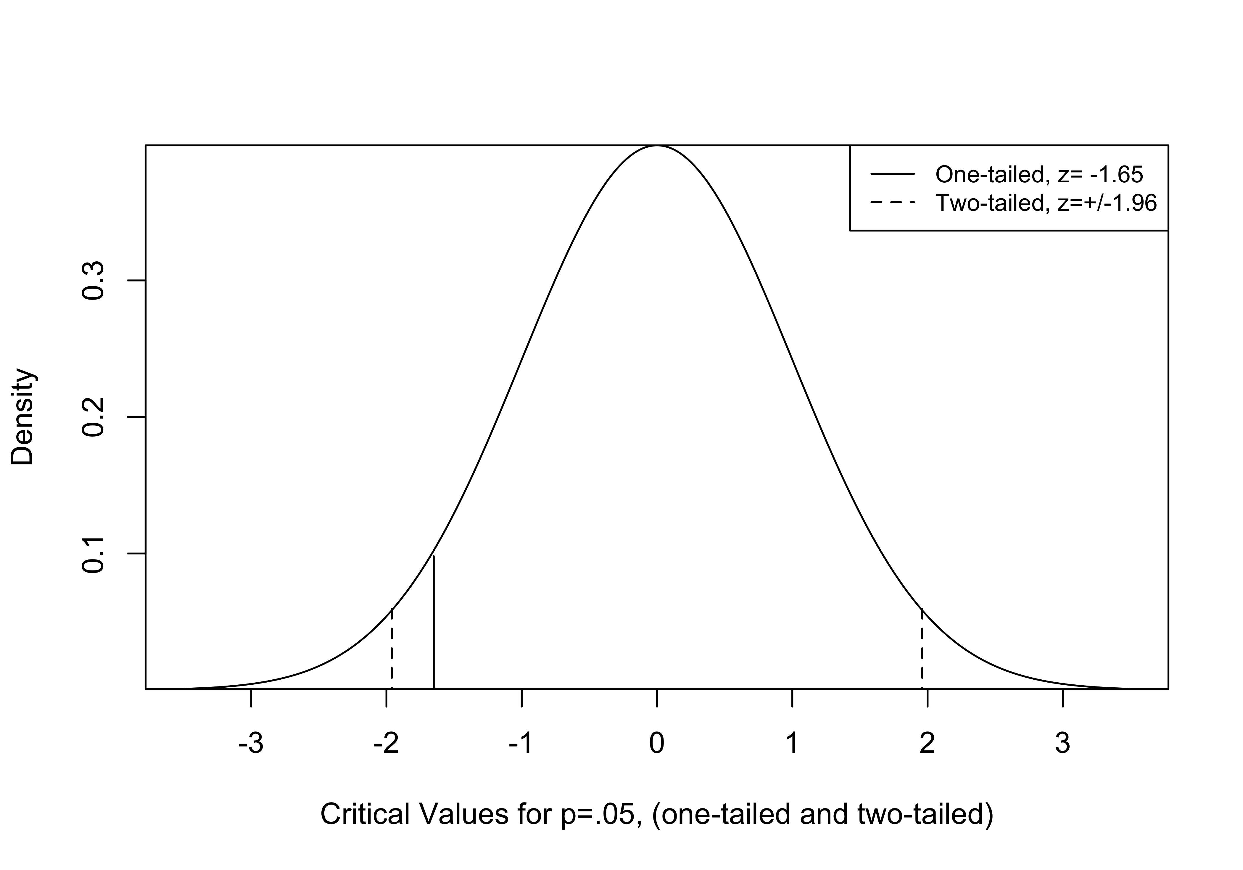
Figure 9.3: Critical Values for One and Two-tailed Tests

The Figure 9.3 illustrates the difference in critical values for one- and two-tailed hypothesis tests. Since we are splitting .05 between the two tails, the c.v. for a two-tailed test is now the z-score that gives us .025 as the area beyond z at the tails of the distribution. Using the qnorm function in R (below), we see that this is z= -1.96, which we take as $\pm 1.96$ for a two-tailed test critical value (p=.05).

[Figure******** 9.3 ********about here]

#Z-score for .025 area at one tail of the distribution
qnorm(.025)

[1] -1.959964

If we obtain a z-score (positive or negative) that is larger in absolute magnitude than this, we reject H₀. Using a two-tailed test requires a larger z-score, making it slightly harder to reject the null hypothesis. However, since the z-score in the sick leave example was -2.86, we would still reject H₀ under a two-tailed test.

In truth, the choice between a one- or two-tailed test rarely makes a difference in rejecting or failing to reject the null hypothesis. The choice matters most when the p-value from a one-tailed test is greater than .025 but less than .05 (just barely into the rejection area), in which case it would be greater than .05 in a two-tailed test. It is worth scrutinizing findings from one-tailed tests that are just barely statistically significant to see if a two-tailed test would be more appropriate. Because it provides a more conservative basis for rejecting the null hypothesis, researchers often choose to report two-tailed significance levels even when a one-tailed test could be justified. Many statistical programs, including R, report two-tailed p-values by default.

T-Distribution

Thus far, we have focused on using z-scores and the z-distribution for testing hypotheses and constructing confidence intervals. Another distribution available to us is the t-distribution. The t-distribution has an important advantage over the z-distribution: it does not assume that we know the population standard error. This is very important because we rarely know the population standard error. In other words, the t-distribution assumes that we are using an estimate of the standard error. As shown in Chapter 8, the estimate of the standard error of the mean is:

\[S_{\bar{x}}=\frac{S}{\sqrt{N}}\]

$S_{\bar{x}}$ is our best guess for $\sigma_{\bar{x}}$, but it is based on a sample statistic, so it does involve some level of error.

To account for the fact that we are estimating the standard error with sample data rather than the population, the t-distribution is somewhat flatter (see Figure 9.4 below) than the z-distribution. Comparing the two distributions, you can see that they are both perfectly symmetric but that the t-distribution is a bit more squat and has slightly fatter tails. This means that the critical value for a given level of significance will be larger in magnitude for a t-score than for a z-score. This difference is especially noticeable for small samples and virtually disappears for samples greater than 100, at which point the t-distribution becomes almost indistinguishable from the z-distribution (see Figure 9.5).

[Figure************************ 9.4 ************************about here]

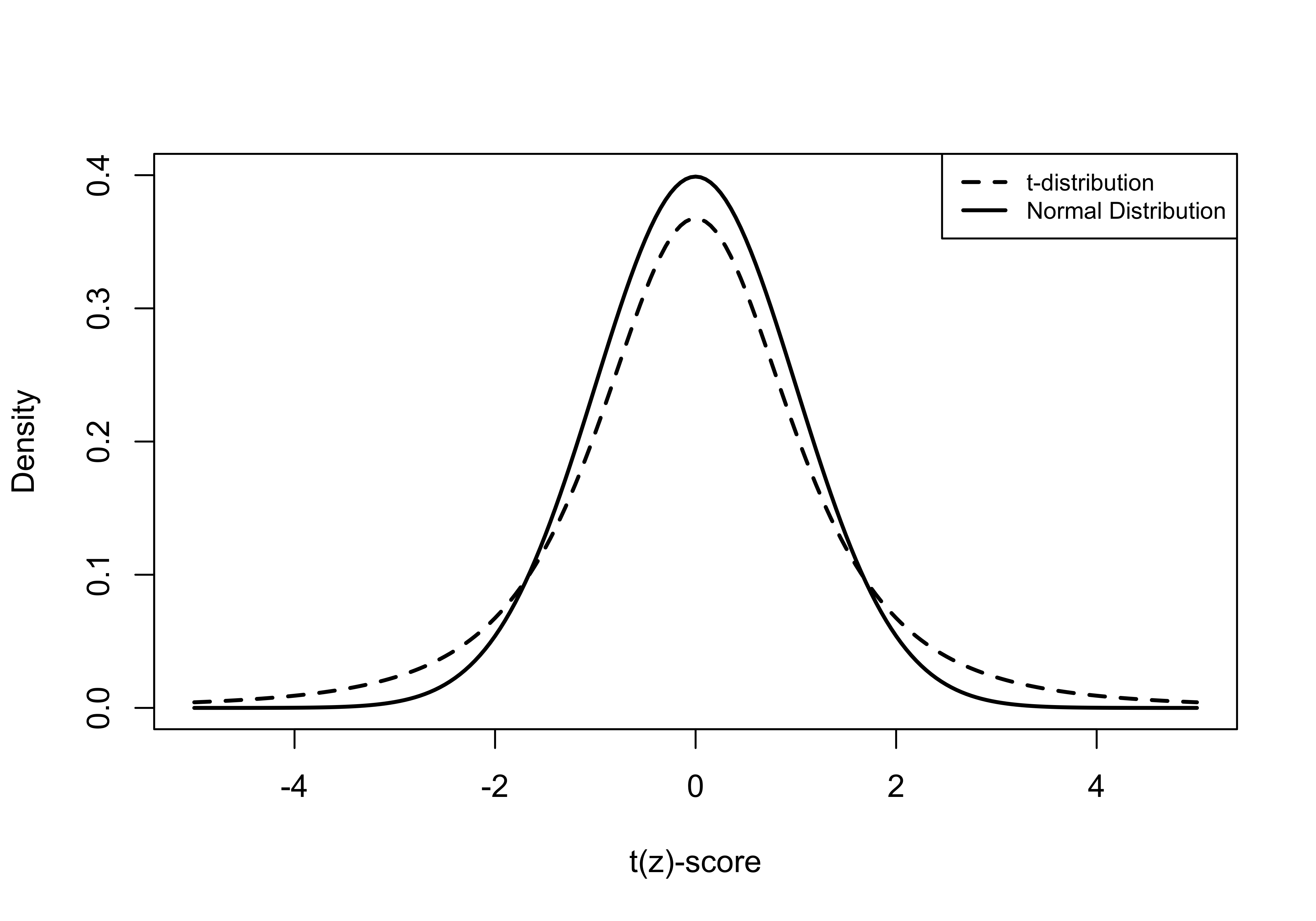
Figure 9.4: Comparison of Normal and t-Distributions

Now, here’s the fun part—the t-score is calculated the same way as the z-score.

\[t=\frac{\bar{x}-\mu}{S_{\bar{x}}}\]

We use the t-score and the t-distribution in the same way and for the same purposes that we use the z-score: choose a desired level of significance (p-value), find the critical value for the t-score, calculate the t-score, and compare the t-score to the critical value, make a decision about the null hypothesis.

While everything here looks about the same as the process for hypothesis testing with z-scores, determining the critical value for a t-distribution is somewhat different and depends upon sample size. This is because we have to consider something called degrees of freedom (df). Taking degrees of freedom into account addresses an issue discussed in Chapter 8, that sample data tend to slightly underestimate the variance and that this underestimation is a bigger problem with small samples. For testing hypotheses about a single mean, degrees of freedom equal:

\[df=n-1\]

So for the sick leave example used above:

\[df=100-1=99\]

You can see the impact of sample size (through degrees of freedom) on the shape of the t-distribution in Figure 9.5: as sample size and degrees of freedom increase, the t-distribution grows more and more similar to the normal distribution. At df=100 (not shown here) the t-distribution is virtually indistinguishable from the z-distribution.

[Figure************************ 9.5 ************************about here]

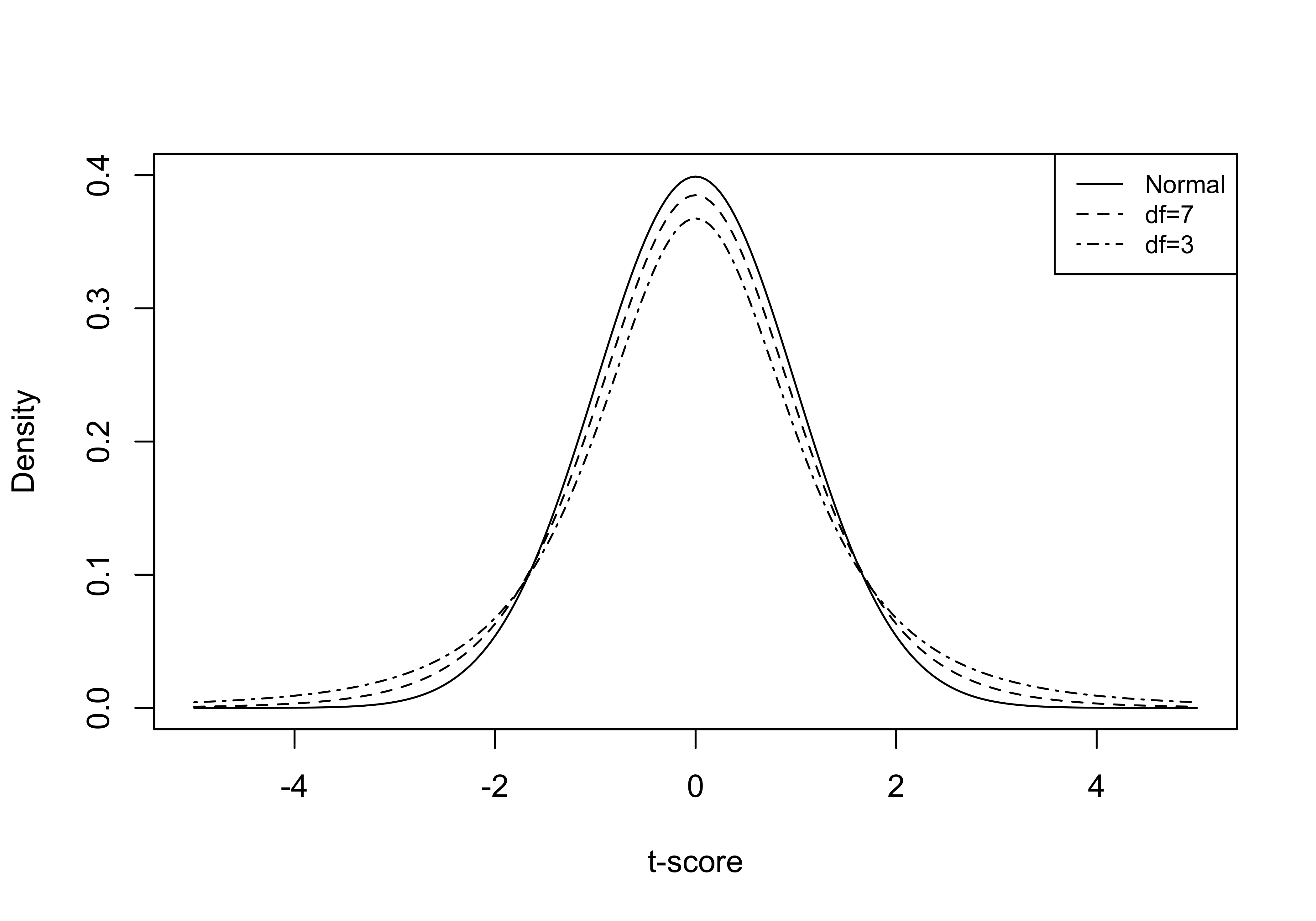
Figure 9.5: Degrees of Freedom and Resemblance of t-distribution to the Normal Distribution

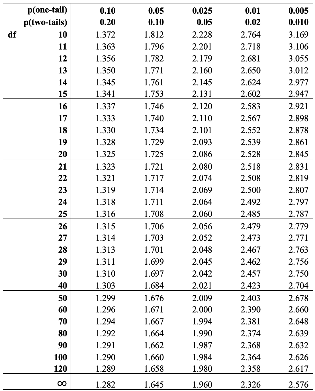
There are two different methods you can use to find the critical value of t for a given level of degrees of freedom. You can go “old school” and look it up in a t-distribution table (Table 9.1),²⁴ or you can ask R to figure it out for you. It’s easier to rely on R for this, but there is some benefit to going old school at least once. In particular, it helps reinforce how degrees of freedom, significance levels, and critical values fit together. You should follow along.

The first step is to decide if you are using a one-tailed or two-tailed test, and then decide what the desired level of significance (p-value) is. For instance, for the sick leave policy example, we can assume a one-tailed test with a .05 level of significance. The relevant column of the table is found by going across the top row of p-values to the column headed by .05. Then, scan down the column until we find the point where it intersects with the appropriate degree of freedom row. In this example, df=99, but there is no listing of df=99 in the table so we will err on the side of caution and use the next lowest value, 90. The .05 one-tailed level of significance column intersects with the df=90 row at t=1.662, so -1.662 is the critical value of t in the sick leave example. Note that it is only slightly different than the c.v. for z that we used in the sick leave calculations, -1.65. This is because the sample size is relatively large (in statistical terms) and the t-distribution closely approximates the z-distribution for large samples. So, in this case the z- and t-distributions lead to the same outcome, we decide to reject H₀.

[Table 9.1 about here]

Table 9.1. T-score Critical Values at Different P-values and Degrees of Freedom

Alternatively, we could ask R to provide this information using the qt function. For this, you need to declare the desired p-value and specify the degrees of freedom, and R reports the critical value:

#Calculate t-score for .05 at the lower tail, with df=99
#The command is: qt(alpha, df)
qt(.05, 99)

[1] -1.660391

By default, qt() provides the critical values for a specified alpha area at the lower tail of the distribution (hence, -1.66). To find the t-score associated with an alpha area at the right (upper) tail of the distribution, just add lower.tail=F to the command:

#Specifying "lower.tail=F" instructs R to find the upper tail area.
qt(.05, 99, lower.tail = F)

[1] 1.660391

For a two-tailed test, you need to cut the alpha area in half, because you are splitting .05 between two tails:

#Calculate t-score for .025 at one tail, with df=99
qt(.025, 99)

[1] -1.984217

Here, R reports a critical value of $-1.984$, which we take as $\pm 1.984$ for a two-tailed test from a sample with df=99. Again, this is slightly larger than the critical value for a z-score (1.96). If you used the t-score table to do this the old-school way, you would find the critical value is t=1.99, for df=90. The results from using the qt function are more accurate than from using the t-table since you are able to specify the correct degrees of freedom.

Whether using a one- or two-tailed test, the conclusion for the sick leave example is unaffected: the t-score obtained from the sample (-2.68) is in the critical region, so reject H₀.

We can also get a bit more precise estimate of the probability of getting a sample mean of 54.8 from a population in which $\mu$=59.2 by using the pt() function to get the area under the curve to the left of t=-2.86:

pt(-2.86, df=99)

[1] 0.002583714

Note that this result is very similar to what we obtained when using the z-distribution (.002118). To get the area under the curve to the right of a positive t-score, add lower.tail=F to the command:

#Specifying "lower.tail=F" instructs R to find the area to the right of
#the t-score
pt(2.86, df=99, lower.tail = F)

[1] 0.002583714

For a two-tailed test using the t-distribution, we double this to find a p-value equal to .005167.

Proportions

As discussed in Chapter 8, the logic of hypothesis testing about mean values also applies to proportions. For example, in the sick leave example, instead of testing whether $\mu=59.2$ we could test a hypothesis regarding the proportion of employees who take a certain number of sick days. Let’s suppose that in the year before the new policy went into effect, 50% of employees took at least 7 sick days. If the new policy has an impact, then the proportion of employees taking at least 7 days of sick leave during the year after the change in policy should be lower than .50. In the sample of 100 employees used above, the proportion of employees taking at least 7 sick days was .41. In this case, the null and alternative hypotheses are:

H₀: P=.50

H₁: P<.50

To review, in the previous example, to test the null hypothesis we established a desired level of statistical significance (.05), determined the critical value for the t-score (-1.66), calculated the t-statistic, and compared it the critical value. There are a couple of differences, however, when working with hypotheses about the population value of proportions.

Because we can calculate the population standard deviation based on the hypothesized value of P (.5), we can use the z-distribution rather than the t-distribution to test the null hypothesis. This is kind of a confusing point. Because the hypothesis is telling us what the population proportion is, it is also, by default, telling us the value of the population standard deviation. If the population value is .50, then the population standard deviation is $\sqrt{P(1-P)}$ and the standard error can be calculated as:

\[S_{p}=\sqrt{\frac{P(1-P)}{n}}= {\sqrt{\frac{.5(.5))}{100}}}=.05\]

Since this is the based the hypothesized population standard deviation, we use a z-score, calculated as before:

\[z=\frac{p-P}{S_{p}}\] Using the data from the problem, this gives us:

\[z=\frac{p-P}{S_{p}}=\frac{.41-.5}{.05}=\frac{-.09}{.05}=-1.8\]

We know from before that the critical value for a one-tailed test using the z-distribution is -1.65. Since this z-score is larger (in absolute terms) than the critical value, we can reject the null hypothesis and conclude that the proportion of employees using at least 7 days of sick leave per year is lower than it was in the year before the new sick leave policy went into effect.

Again, we can be a bit more specific about the p-value:

pnorm(-1.8)

[1] 0.03593032

Here are a couple of things to think about with this finding. First, while the p-value is lower than .05, it is not much lower. In this case, if you took 1000 samples of 100 workers from a population in which $P=.50$ and calculated the proportion who took 7 or more sick days, approximately 36 of those samples would produce a proportion equal to .41 or lower, just due to sampling error. This still means that the probability of getting this sample finding from a population in which the null hypothesis was true is pretty small (.03593), so we should be comfortable rejecting the null hypothesis. But what if there were good reasons to use a two-tailed test? Would we still reject the null hypothesis? No, because the critical value for a two-tailed test (-1.96) would be larger in absolute terms than the z-score, and the p-value would be .07186. These findings stand in contrast to those from the analysis of the average number of sick days taken, where the p-values for both one- and two-tailed tests were well below the .05 cut-off level.

One of the take-home messages from this example is that confidence in research findings is sometimes fragile, since “significance” can be a function of how you frame the hypothesis test (one- or two-tailed test?) or how you measure your outcomes (average hours of sick days taken, or proportion who take a certain number of sick days). For this reason, it is always a good idea to be mindful of how the choices you make might influence your findings.

Types of Error

In both the difference in means and difference in proportions tests above, we concluded that there was decrease in the use of sick leave in the year following the implementation of the new sick leave policy. Based on the p-values from the hypothesis tests, we rejected the null hypotheses, concluding that there was small enough probability of getting the sample findings from a population in which H₀ was true, that it was unlikely to be true.

But what if we are wrong? What if there actually was no change in sick leave usage in the year following the implementation of the new policy but we concluded there was? Is this possible? Yes, it is possible to make errors like this when testing hypotheses. Generally, we think of these types of errors as Type I and Type II errors, as described Figure 9.6.

In the current example, we rejected H₀ and concluded, based on sample findings, that there was a significant decline in sick leave useage in the year following the the implementation of a new sick leave policy. If, in the population, the null hypothesis were actually true (there was no change in sick leave use), then we would be making a Type I error, rejecting H₀ when it is true. This is also referred to as an alpha ($\alpha$ ) error, because the probability of committing a Type I error is equal to the p-value used to decide if the null hypothesis should be rejected. In both cases explored above, we used a .05 threshold for rejection, but we also know from the p-values associated with the t-scores that the probability of making a Type I error is .0359 for the difference in proportions test, and .0052 for the difference in means test. Given this, we know that the probability of making a Type I error is low.

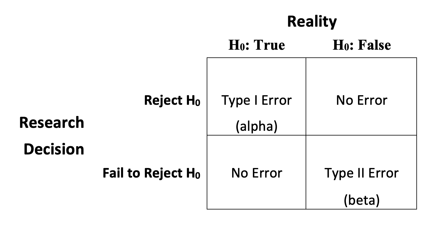
Figure 9.6: Potential Errors in Hypothesis Testing

[Figure******** 9.6 ********about here]

The other type of error that can occur in hypothesis testing is Type II, or beta ($\beta$ ) error, where you fail to reject H₀ even though it is false. Suppose in the sick leave example, we had decided that we wanted to be very certain before rejecting H₀, so we decided to use a p-value of .01 as the threshold for rejection instead of .05. In that case, we would have failed to reject H₀ in the difference in proportions test since the p-value there was .0359. By requiring a smaller p-value, we decreased the probability of a Type I error, but increased the likelihood of committing a Type II error, concluding that the sick leave policy had no impact when in fact it did. This illustrates that the two types of errors are inversely related to each other: as the probability of Type I error decreases, perhaps by requiring smaller p-values before rejecting H₀, the probability of Type II increases.

One way to minimize both Type I and Type II error is to increase the sample size. If you are able to control the size of the sample, moving from small to reasonably large samples pays dividends, as shown in Chapter 8.

T-test in R

Let’s say you are looking at data on public perceptions of the presidential candidates in 2020 and you have a sense that people had mixed feelings about Democratic nominee, Joe Biden, going into the election. This leads you to expect that his average rating on the 0 to 100 feeling thermometer scale from the ANES was probably about 50. You decide to test this directly with the anes20 data set.

The null hypothesis is:

H₀: $\mu=50$

Because there are good arguments for expecting the mean to be either higher or lower than 50, the alternative hypothesis is two-tailed:

H₁: $\mu\ne50$

First, you get the sample mean:

#Get the sample mean for Biden's feeling thermometer rating
mean(anes20$V202143, na.rm=T)

[1] 53.41213

Here, you see that the mean feeling thermometer rating for Biden in the fall of 2020 was 53.41. This is higher than what you thought it would be (50), but you know that it’s possible to could get a sample outcome of 53.41 from a population in which the mean is actually 50, so you need to do a t-test to rule out sampling error as reason for the difference.

In R, the command for a one-sample two-tailed t-test is relatively simple, you just have to specify the variable of interest and the value of $\mu$ under the null hypothesis:

#Use 't.test' and specify the variable and mu
t.test(anes20$V202143, mu=50)


    One Sample t-test

data:  anes20$V202143
t = 8.1805, df = 7368, p-value = 3.303e-16
alternative hypothesis: true mean is not equal to 50
95 percent confidence interval:
 52.59448 54.22978
sample estimates:
mean of x 
 53.41213

These results are pretty conclusive, the t-score is 8.2 and the p-value is very close to 0.²⁵ Also, if it makes more sense for you to think of this in terms of a confidence interval, the 95% confidence interval ranges from about 52.6 to 54.2, which does not include 50. You should reject the null hypothesis and conclude instead that Biden’s feeling thermometer rating in the fall of 2020 was greater than 50.

Even though Joe Biden’s feeling thermometer rating was greater than 50, from a substantive perspective it is important to note that a score of 53 does not mean Biden was wildly popular, just that his rating was greater than 50. This highlights an important thing to remember: statistically significant results are not necessarily substantively large results. This point is addressed at greater length in the next several chapters, where we explore measures of substantive importance that can be used to complement measures of statistical significance.

Next Steps

The last three chapters have given you a foundation in the principles and mechanics of sampling, statistical inference, and hypothesis testing. Everything you have learned thus far is interesting and important in its own right, but what is most exciting is that it prepares you for testing hypotheses about outcomes of a dependent variable across two or more categories of an independent variable. In other words, you now have the tools necessary to begin looking at relationships among variables. We take this up in the next chapter by looking at differences in outcomes across two groups. Following that, we test hypotheses about outcomes across multiple groups in Chapters 11 through 13. In each of the next several chapters, we continue to focus on methods of statistical inference, exploring alternative ways to evaluate statistical significance. At the same time, we also introduce the idea of evaluating the strength of relationships by focusing on measures of effect size. Both of these concepts–statistical significance and effect size–continue to play an important role in the remainder of the book.

Exercises

Concepts and Calculations

The survey of 300 college students introduced in the end-of-chapter exercises in Chapter 8 found that the average semester expenditure was $350 with a standard deviation of $78. At the same time, campus administration has done an audit of required course materials and claims that the average cost of books and supplies for a single semester should be no more than $340. In other words, the administration is saying the population value is $340.
1. State a null and alternative hypothesis to test the administration’s claim. Did you use a one- or two-tailed alternative hypothesis? Explain your choice.
2. Test the null hypothesis and discuss the findings. Show all calculations.
The same survey reports that among the 300 students, 55% reported being satisfied with the university’s response to the COVID-19 pandemic. The administration hailed this finding as evidence that a majority of students support the course they’ve taken in reaction to the pandemic. (Hint: this is a “proportion” problem)
1. State a null and alternative hypothesis to test the administration’s claim. Did you use a one- or two-tailed alternative hypothesis? Explain your choice
2. Test the null hypothesis and discuss the findings. Show all calculations
Determine whether the null hypothesis should be rejected for the following pairs of t-scores and critical values.
1. t=1.99, c.v.= 1.96
2. t=1.64, c.v.= 1.65
3. t=-2.50, c.v.= -1.96
4. t=1.55, c.v.= 1.65
5. t=-1.85, c.v.= -1.96
A researcher at the county elections office was interested in whether voter turnout in the county had changed significantly since the last election, when it was 59%. They were impatient and didn’t want to tabulate all of the precincts, so they took a random sample of 100 precincts and found that turnout in the sample of precincts was 53%. The t-score for the difference is -2.02 and the p-value was .023.
1. In this example, is the research testing a one- or two-tailed hypothesis?
2. What is the value of $\mu$ ?
3. Does the evidence here support rejecting the null hypothesis that there is no change in turnout?
4. What is the probability of committing a Type I error in this example?
5. Suppose the researcher decides to use a .01 instead of .05 threshold for rejecting the null hypothesis. Does this affect the probability of making Type I and Type II errors? Explain.

R Problems

For the first three questions, use the feeling thermometers for Donald Trump (anes20$V202144), liberals (anes20$V202161), and conservatives (anes20$V202164).

Using descriptive statistics and either a histogram, boxplot, or density plot, describe the central tendency and distribution of each feeling thermometer.
Use the t.test function to test the null hypotheses that the mean for each of these variables in the population is equal to 50. State the null and alternative hypotheses and interpret the findings from the t-test.
Taking these findings into account, along with the analysis of the Joe Biden’s feeling thermometer at the end of the chapter, do you notice any apparent contradictions in American public opinion? Explain.
Use the pt() function to calculate the p-value (area at the tail) for each of the following t-scores (assume one-tailed tests).
1. t=1.45, df=49
2. t=2.11, df=30
3. t=-.69, df=200
4. t=-1.45, df=100
What are the p-values for each of the t-scores listed in Problem 4 if you assume a two-tailed test?
Treat the t-scores from Problem 4 as z-scores and use the pnorm() to calculate the p-values. List the p-values and comment on the differences between the p-values associated with the t- and z-scores. Why are some closer in value than others?

The code for generating this table comes from Ben Bolker via stackoverflow (https://stackoverflow.com/questions/31637388/).↩︎
Remember that 3e-16 is scientific notation and means that you should move the decimal point 16 places to the left of 3. This means that p=.0000000000000003.↩︎