Resampling & cross-validation

Learning outcomes/objective: Learn…

…why resampling is helpful.
…how to use resampling to evaluate accuracy and avoid overfitting.

Sources: James et al. (2013) (Ch. 5); Fit a model with resampling;

1 Retake: Datasets in ML

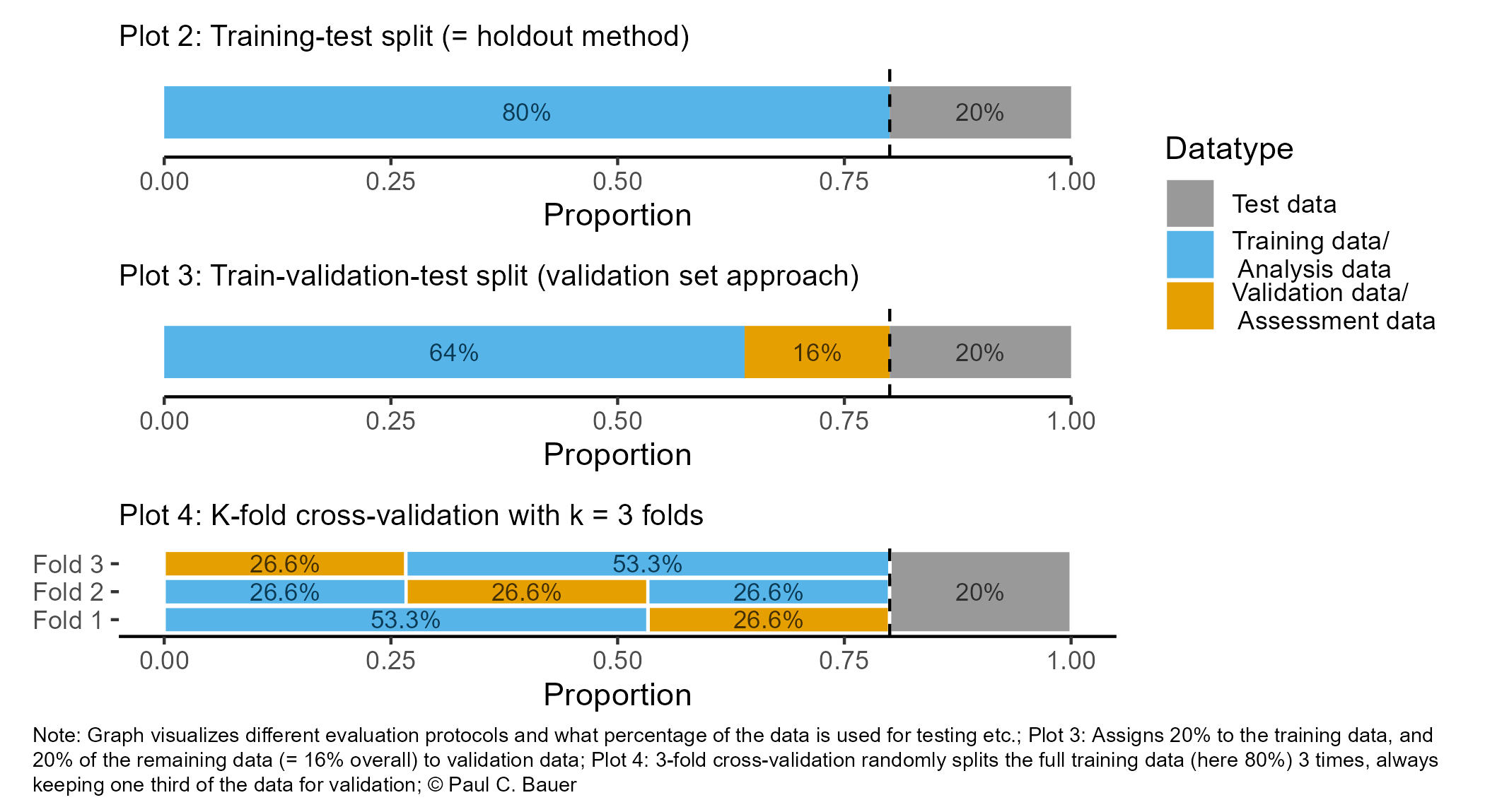
Figure 1: Different datasets in machine learning (Source: Own illustration)

So far we pursued the strategy Figure 1, Plot 2.
Plot 3 illustrates the strategy, where we do a 2nd split into training (analysis)/validation (assessment data).
- This allows us to iterate over training/validating model (e.g., for parameter tuning) keeping the test data for a final test.
Q1: What could be disadvantages the approaches in Plot 1 (and 2) in Figure 1 when building a predictive model? Consider the randomness in splits.
Q2: How could the size of training and test data (and validation data) affect representativeness?
Q3: James et al. (2013) use Figure 5.1 [p.177] to explain the validation set approach (= single split). Please inspect the figure and explain it in a few words.

Insights

Q1: Disadvantages of a single split: Estimate of test error rate can be highly variable, depending on which observations included in train data/test data.
- The same is true if we further split into training and validation data. We are doing a second split here but through chance we could end up with a training/validation datasets that somehow are non-typical (and badly generalize to the test dataset).
Q2: A small training dataset may not adequately represent the underlying distribution of the data (sample representativeness), leading to biased estimates of model parameters. In contrast, a larger training dataset is more likely to capture the true distribution of the data, reducing bias in the model.
Q3: See book!

2 Splitting the data and overfitting

To avoid overfitting we can estimate our model based on different resamples as shown in Figure 2
- Datasets obtained from the initial split are called training and test data (also hold out set)
- Datasets obtained from further splits to the training data are called analysis (training) and assessment (validation) datasets
  - We call such further splits folds and we resample for each fold (below we have B folds)

Figure 2: Source: https://bookdown.org/max/FES/resampling.html

3 Resampling methods (1)

Resampling methods (James et al. 2013, Ch. 5)
- Repeatedly draw samples from training (analysis) set and refit model of interest on each sample to obtain additional information about the fitted model, e.g., the variability of a logistic regression fit
- Aim: Obtain information that would not be available from fitting model only once using the original training sample
Model assessment: Process of evaluating a model’s performance
Model selection: Process of selecting the proper level of flexibility for a model
Common resampling methods: Cross-validation (CV) and bootstrap
- Cross-validation used to (1) estimate the test error associated with a given statistical learning method in order to evaluate its performance, or (2) to select the appropriate level of model flexibility
- Bootstrap most commonly used in model selection to provide a measure of accuracy of a parameter estimate or of a given statistical learning method
Here we discuss cross-validation!

4 Resampling methods (2): Cross-validation

Recap: Training error rate vs. test error rate (James et al. 2013, chap. 2.2.3)
- “test error is the average error that results from using a statistical learning method to predict the response on a new observation – that is, a measurement that was not used in training the method” (James et al. 2013, 176)
Objective: Estimate this test error
- i.e., prediction errors our model would make for new data, e.g., for prisoners that were not used to train the model
In absence of large designated test set a number of techniques can be used to estimate test error rate using the available training data (James et al. 2013, 176)
Cross-validation (CV) (James et al. 2013, chap. 5.1)
- Class of methods to estimate test error rate by holding out a subset of the training observations from the fitting process, and then applying the statistical learning method to those held out observations
- James et al. (2013) discuss CV for regression approach [Ch. 5.1.1-5.1.4] and classification approach [Ch. 5.1.5]

5 Resampling methods (3): Leave-one-out cross-validation (LOOCV)

Q: James et al. (2013) use Figure 5.3 [p.179] to explain the Leave-One-Out Cross-Validation (LOOCV). Please inspect the figure and explain it in a few words.
Q: What is shown in Figure 3?

Figure 3: Leave-one-out cross-validation (LOOCV): With n = 8 observations a total of 8 models will be trained and tested (Source: MBanuelos22/Wikipedia (CC BY-SA 4.0))

Data set repeatedly split into two parts, whereby a single observation \((x_{1},y_{1})\) is used for assessment (validation dataset)
- Remaining observations \({(x_{2},y_{2}),...,(x_{n},y_{n})}\) make up the analysis (training) dataset
- Statistical learning method is fit on the \(n−1\) training observations and prediction is made for excluded observation
- Repeated for all splits
Q: What might be advantages/disadvantages of LOOCV? Bias? Reproducibility? Computational intensity?

Insights

Advantages over validation set approach
- Bias: Less bias across assessment/training datasets because they are bigger (Why?)
- Reproducibility: Performing LOOCV repeatedly will always produces the same results
  - Why? No randomness in training/validation set splits.. we use all possible splits
Computational intensity: Disadvantage: Can be computationally intensive (Why?) [estimate it n times]

6 Resampling methods (4): Leave-one-out cross-validation (LOOCV)

In classification setting LOOCV error rate takes the form (James et al. 2013, 184):

\[CV_{(n)} = \frac{1}{n}\sum_{i=1}^{n}Err_{i}\] where \(Err_{i}=I(y_{i}\neq\hat{y}_{i})\), i.e., is 1 when left-out \(y_{i}\) was wrongly predicted

Linear regression: Use MSE rather than number of misclassified observations to quantify test error
The k-fold CV error rate (see next slide) and validation set error rates are defined analogously

7 Resampling methods (5): k-Fold Cross-Validation

James et al. (2013) use Figure 5.5 [p.179] to explain the k-Fold Cross-Validation. Please inspect the figure and explain it in a few words.
Q: What is shown in Figure 4?

Figure 4: K-fold cross-validation: With n = 12 observations and k = 3 folds, data will be shuffled and a total of 3 models trained and tested (Source: MBanuelos22/Wikipedia (CC BY-SA 4.0))

k-Fold Cross-Validation is special case of LOOCV where \(k\) is set to equal \(n\)
Error rate: \(CV_{(k)} = \frac{1}{k}\sum_{i=1}^{k}Err_{i}\)
Q1: What is the advantage of using \(k = 5\) or \(k = 10\) rather than \(k = n\)?
Q2: Imagine our full training dataset has \(n = 5000\) observations and we use crossvalidation with \(k = 5\) and \(k = 10\). How many observations will we have in the respective analysis/assessment datasets of the respective resample?
Q3: k-Fold CV may give more accurate estimates of test error rate than LOOCV: Why? (cf. Bias-variance trade-off, James et al. (2013), Ch. 5.1.4)

Answers

Q1: Less computationally intensive
Q2:
- \(k = 5 \rightarrow 5000/5 \rightarrow n_{\text{analysis/training}} = 4000 \text{ and } n_{\text{assessment/validation}} = 1000\)
- \(k = 10 \rightarrow 5000/10 \rightarrow n_{\text{analysis/training}} = 4500 \text{ and } n_{\text{assessment/validation}} = 500\)
Q3: Bias-variance trade-off (James et al. 2013, Ch. 5.1.4)
- Datasets smaller than LOOCV, but larger than validation set approach
  - LOOCV best from bias perspective but (most observations) but each model fit on identical observations (predictions highly correlated)
    - Mean of many highly correlated quantities has higher variance than does the mean of many quantities that are not as highly correlated → test error estimate from LOOCV higher variance than test error estimate from k-fold CV (variance inflation phenomenon¹)
Recommendation use k-fold cross-validation using k = 5 or k = 10

8 Resampling methods (6): Some caveats

Beware: Conceptual confusion
- Cross-validation four meanings in political science (Neunhoeffer and Sternberg 2019, 102)
  - 1. Validating new measures or instruments
  - Resampling:
    - 1. Robustness check of coefficents across data subsets
    - 1. procedure to obtain estimate of true error (unseen data)
    - 1. procedure of model tuning (e.g., parameter tuning, feature selection, up-/down-sampling of imbalanced data prior to training)
Cross-validation for tuning vs. test error rate
- “A problematic use of cross-validation occurs when a single cross-validation procedure is used for model tuning and to estimate true error at the same time […]. Ignoring this can lead to serious misreporting of performance measures. If the goal of cross-validation is to obtain an estimate of true error, every step involved in training the model (including (hyper-) parameter tuning, feature selection or up-/down-sampling) has to be performed on each of the training folds of the cross-validation procedure. Hastie, Tibshirani, and Friedman (2011, 245) refer to this problem as the wrong way of doing cross-validation. We take down-sampling of imbalanced data as a simple example of this problem.” (Neunhoeffer and Sternberg 2019, 102)

9 Exercise: Resampling methods

Let’s quickly review cross-validation
1. Why/when do we normally use cross-validation (“resampling methods”)?
2. Explain how k-fold cross-validation is implemented.
3. What are the advantages and disadvantages of k-fold cross-validation relative to the validation set approach?
4. What are the advantages and disadvantages of k-fold cross-validation relative to LOOCV?

Answers

Cross-validation, or resampling methods, are typically used in machine learning for model evaluation, hyperparameter tuning, and to estimate the model’s performance on unseen data. It helps to mitigate issues such as overfitting and provides a more robust estimate of the model’s generalization ability compared to a single train-test split.
K-fold cross-validation involves dividing the dataset into k equal-sized folds. The model is trained k times, each time using k-1 folds for training and the remaining fold for validation. This process is repeated k times, with each fold serving as the validation dataset exactly once. The performance metrics are then averaged across the k iterations to obtain the final performance estimate.
Advantages: more reliable estimate of the model’s performance; utilizes the entire dataset for both training and validation, reducing the risk of bias; Disadvantages: requires more computational resources; may be less suitable for large datasets
Advantages: Less computationally intensive; Provides a good balance between bias and variance; Disadvantages: May be biased if the dataset contains significant class imbalances or if the data is not uniformly distributed across folds; May underestimate true error rate if the dataset is small or if the model is unstable

10 Tidymodels: Resampling

rsample: for sample splitting (e.g. train/test or cross-validation)
- provides functions to create different types of resamples and corresponding classes for their analysis
initial_split: Use this to split the data into training and test data (with arguments prop, strata)
- prop-argument: Specify share of training data observations
- strata-argument: Conduct stratified sampling on the dependent variable (better if classes are imbalanced!)
initial_validation_split(data, prop = c(0.6, 0.2)): Split into training (60%), validation (20%), and test data (20%)
vfold_cv(data_train, v = 10): randomly splits the data into \(v = k\) groups of roughly equal size (called “folds”)
- Use after initial_split, i.e., split into training/test data
- fit_resamples() (tune package): computes a set of performance metrics across one or more resamples
training(), testing(), analysis() and assessment() can be used to extract the corresponding datasets from an rsplit object

11 Lab: Evaluate a classification model using training, validation and test dataset

See here for a description of the data and illustration of how to explore the data.

We first import the data into R:

# install.packages(pacman)
pacman::p_load(tidyverse,
               tidymodels,
               knitr,
               kableExtra,
               DataExplorer,
               visdat,
               naniar)

rm(list=ls())
load(url(sprintf("https://docs.google.com/uc?id=%s&export=download",
                         "1gryEUVDd2qp9Gbgq8G0PDutK_YKKWWIk")))

Steps:

Split data into training, validation and test data.
Define the recipe & model
Bundle the model/formula into a workflow
Fit the workflow on the training data and evaluate on validation data -> if not happy change workflow/recipe/model
If happy with the accuracy estimate model on complete training dataset (analysis + assessment) and evaluate accuracy in test data (holdout dataset)

# Extract data with missing outcome
  data_missing_outcome <- data %>% filter(is.na(is_recid_factor))
  dim(data_missing_outcome)

[1] 614  14

# Omit individuals with missing outcome from data
  data <- data %>% drop_na(is_recid_factor) # ?drop_na
  dim(data)

[1] 6600   14

# 1.
# Split the data into training, validation and test data
  set.seed(1234)
  data_split <- initial_validation_split(data, prop = c(0.6, 0.2))
  data_split # Inspect

<Training/Validation/Testing/Total>
<3960/1320/1320/6600>

# Extract the datasets
  data_train <- training(data_split)
  data_validation <- validation(data_split)
  data_test <- testing(data_split) # Do not touch until the end!
  dim(data_train)

[1] 3960   14

  dim(data_validation)

[1] 1320   14

  dim(data_test)

[1] 1320   14

# 2.
# Define the recipe & model
  recipe1 <- recipe(is_recid_factor ~ age + priors_count + 
                      sex + race, data = data_train)
  
  model1 <- logistic_reg() %>% 
    set_engine("glm") %>% # lm engine
    set_mode("classification") # regression problem
  
# 3.
# Create workflow
  workflow1 <- 
  workflow() %>% 
  add_model(model1) %>%
  add_recipe(recipe1)

# 4. Fit the workflow on training set & accuracy
  fit_train <- workflow1 %>% fit(data = data_train)

  data_train <- augment(fit_train, data_train, 
                        type.predict = "response") 

  data_train %>%
      metrics(truth = is_recid_factor, estimate = .pred_class)

# A tibble: 2 × 3
  .metric  .estimator .estimate
  <chr>    <chr>          <dbl>
1 accuracy binary         0.673
2 kap      binary         0.344

  # Predict & assess metrics in validation set
  augment(fit_train, data_validation, # Make sure to use training fit!
          type.predict = "response") %>%
      metrics(truth = is_recid_factor, estimate = .pred_class)

# A tibble: 2 × 3
  .metric  .estimator .estimate
  <chr>    <chr>          <dbl>
1 accuracy binary         0.670
2 kap      binary         0.336

# 5. If happy fit workflow on full 
  # training set (data_train + data validation) 
  # and predict values on test set
  data_training_full <- bind_rows(data_train, data_validation)
  fit_train_full <- workflow1 %>% fit(data = data_training_full)
  
  # Predict and assess accuracy
  augment(fit_train_full, data_test, 
          type.predict = "response") %>%
      metrics(truth = is_recid_factor, estimate = .pred_class)

# A tibble: 2 × 3
  .metric  .estimator .estimate
  <chr>    <chr>          <dbl>
1 accuracy binary         0.671
2 kap      binary         0.341

12 Lab: Evaluate a classification model with resampling

See here for a description of the data and illustration of how to explore the data.

We first import the data into R:

# install.packages(pacman)
pacman::p_load(tidyverse,
               tidymodels,
               knitr,
               kableExtra,
               DataExplorer,
               visdat,
               naniar)

rm(list=ls())
load(url(sprintf("https://docs.google.com/uc?id=%s&export=download",
                         "1gryEUVDd2qp9Gbgq8G0PDutK_YKKWWIk")))

Steps:

Initial first split of the data
Create resampled partitions/folds with vfold_cv()
Define the recipe & model
Bundle the model/formula into a workflow
Fit the workflow on the resamples/folds & extract accuracy metrics
If happy with the accuracy estimate model on complete training dataset and evaluate accuracy in test data (holdout dataset)

# Extract data with missing outcome
  data_missing_outcome <- data %>% 
                  filter(is.na(is_recid_factor))
  dim(data_missing_outcome)

[1] 614  14

# Omit individuals with missing outcome from data
  data <- data %>% drop_na(is_recid_factor) # ?drop_na
  dim(data)

[1] 6600   14

# 1.
# Split the data into training and test data
  data_split <- initial_split(data, prop = 0.8)
  data_split # Inspect

<Training/Testing/Total>
<5280/1320/6600>

# Extract the two datasets
  data_train <- training(data_split)
  data_test <- testing(data_split) # Do not touch until the end!

# 2.  
# Create resampled partitions of training data
  set.seed(345)
  data_folds <- vfold_cv(data_train, v = 10) # V-fold/k-fold cross-validation
  data_folds # data_folds now contains several resamples of our training data

#  10-fold cross-validation 
# A tibble: 10 × 2
   splits             id    
   <list>             <chr> 
 1 <split [4752/528]> Fold01
 2 <split [4752/528]> Fold02
 3 <split [4752/528]> Fold03
 4 <split [4752/528]> Fold04
 5 <split [4752/528]> Fold05
 6 <split [4752/528]> Fold06
 7 <split [4752/528]> Fold07
 8 <split [4752/528]> Fold08
 9 <split [4752/528]> Fold09
10 <split [4752/528]> Fold10

  # v = 10 -> n/10 gives number of validation set observation in each fold

  
  
# 3.
# Define the recipe & model
  recipe1 <- recipe(is_recid_factor ~ age + priors_count + 
                      sex + race, data = data_train)
  
  model1 <- logistic_reg() %>% 
    set_engine("glm") %>% # lm engine
    set_mode("classification") # regression problem
  
# 4.
# Create workflow
  workflow1 <- 
  workflow() %>% 
  add_model(model1) %>%
  add_recipe(recipe1)

# 5. Fit the workflow on the folds/resamples
  # There is no need in specifying 
  # data_analysis/data_assessment as 
  # the functions understand the corresponding parts
  fit1 <- 
  workflow1 %>% 
  fit_resamples(resamples = data_folds)
  # add argument "control" to keep predictions
    # control = control_resamples(save_pred = TRUE, extract = function (x) extract_fit_parsnip(x))
  
  fit1

# Resampling results
# 10-fold cross-validation 
# A tibble: 10 × 4
   splits             id     .metrics         .notes          
   <list>             <chr>  <list>           <list>          
 1 <split [4752/528]> Fold01 <tibble [2 × 4]> <tibble [0 × 3]>
 2 <split [4752/528]> Fold02 <tibble [2 × 4]> <tibble [0 × 3]>
 3 <split [4752/528]> Fold03 <tibble [2 × 4]> <tibble [0 × 3]>
 4 <split [4752/528]> Fold04 <tibble [2 × 4]> <tibble [0 × 3]>
 5 <split [4752/528]> Fold05 <tibble [2 × 4]> <tibble [0 × 3]>
 6 <split [4752/528]> Fold06 <tibble [2 × 4]> <tibble [0 × 3]>
 7 <split [4752/528]> Fold07 <tibble [2 × 4]> <tibble [0 × 3]>
 8 <split [4752/528]> Fold08 <tibble [2 × 4]> <tibble [0 × 3]>
 9 <split [4752/528]> Fold09 <tibble [2 × 4]> <tibble [0 × 3]>
10 <split [4752/528]> Fold10 <tibble [2 × 4]> <tibble [0 × 3]>

# Extract single components from folds
  fit1$.metrics[1:2] # get first two rows of .metrics

[[1]]
# A tibble: 2 × 4
  .metric  .estimator .estimate .config             
  <chr>    <chr>          <dbl> <chr>               
1 accuracy binary         0.661 Preprocessor1_Model1
2 roc_auc  binary         0.707 Preprocessor1_Model1

[[2]]
# A tibble: 2 × 4
  .metric  .estimator .estimate .config             
  <chr>    <chr>          <dbl> <chr>               
1 accuracy binary         0.693 Preprocessor1_Model1
2 roc_auc  binary         0.749 Preprocessor1_Model1

# 6. 
# Collect metrics across resamples
  collect_metrics(fit1)

# A tibble: 2 × 6
  .metric  .estimator  mean     n std_err .config             
  <chr>    <chr>      <dbl> <int>   <dbl> <chr>               
1 accuracy binary     0.678    10 0.00503 Preprocessor1_Model1
2 roc_auc  binary     0.732    10 0.00582 Preprocessor1_Model1

If we are happy with the average accuracy of our model of 0.68 across resamples we would then use the same model defined above, fit it on the whole (non-splitted) training dataset and create a new fitted model fit2. We can evaluate the accuracy of that new model in the training set and then move to the test data further below.

# 7. 
  # Fit on training dataset (fit2!!!)
  fit2 <- workflow1 %>% fit(data = data_train)

  
# Training data: Add predictions 
  data_train <- augment(fit2, data_train, type.predict = "response") 

  head(data_train %>%
      select(is_recid_factor, age, .pred_class, 
             .pred_no, .pred_yes))

# A tibble: 6 × 5
  is_recid_factor   age .pred_class .pred_no .pred_yes
  <fct>           <dbl> <fct>          <dbl>     <dbl>
1 yes                30 yes            0.293     0.707
2 no                 35 no             0.583     0.417
3 yes                28 no             0.631     0.369
4 no                 37 no             0.644     0.356
5 yes                37 no             0.527     0.473
6 no                 21 yes            0.413     0.587

# Training data: Metrics
  data_train %>%
      metrics(truth = is_recid_factor, estimate = .pred_class)

# A tibble: 2 × 3
  .metric  .estimator .estimate
  <chr>    <chr>          <dbl>
1 accuracy binary         0.679
2 kap      binary         0.356

And finally evaluate the model using the test data (holdout set).

# 8. 
# Test data: Add predictions 
  data_test<- augment(fit2, data_test, type.predict = "response")

  head(data_test %>%
      select(is_recid_factor, age, .pred_class, .pred_no, .pred_yes))

# A tibble: 6 × 5
  is_recid_factor   age .pred_class .pred_no .pred_yes
  <fct>           <dbl> <fct>          <dbl>     <dbl>
1 yes                24 yes            0.334     0.666
2 no                 39 no             0.757     0.243
3 yes                64 yes            0.453     0.547
4 no                 21 no             0.564     0.436
5 yes                26 yes            0.320     0.680
6 yes                33 no             0.598     0.402

# Test data: Metrics
  data_test %>%
      metrics(truth = is_recid_factor, estimate = .pred_class)

# A tibble: 2 × 3
  .metric  .estimator .estimate
  <chr>    <chr>          <dbl>
1 accuracy binary         0.645
2 kap      binary         0.287

# More accuracy metrics
  metrics_combined <- metric_set(accuracy, precision, recall, f_meas)

  # The returned function has arguments:
  data_test %>% 
  metrics_combined(truth = is_recid_factor, estimate = .pred_class)

# A tibble: 4 × 3
  .metric   .estimator .estimate
  <chr>     <chr>          <dbl>
1 accuracy  binary         0.645
2 precision binary         0.647
3 recall    binary         0.686
4 f_meas    binary         0.666

# Cross-classification table
  conf_mat(data = data_test,
           truth = is_recid_factor, estimate = .pred_class)

          Truth
Prediction  no yes
       no  468 255
       yes 214 383

12.0.1 Visual assessment of accuracy

Figure 5 displays the ROC curve (see the corresponding slide for an overview). The corresponding values can be obtained using the roc_curve() function.

Important (?roc_curve): “There is no common convention on which factor level should automatically be considered the”event” or “positive” result when computing binary classification metrics. In yardstick, the default is to use the first level. To alter this, change the argument event_level to “second” to consider the last level of the factor the level of interest.”
- Here we pick the 1s, i.e., recidivating as the “event” or “positive” result.

data_test %>% 
  roc_curve(truth = is_recid_factor, 
            .pred_yes,
            event_level = "second") %>% 
  autoplot() + 
  xlab("1 - specificity (FPR = FP/N, false positives rate)") +
  ylab("sensitivity (TPR = TP/P, true positives rate)")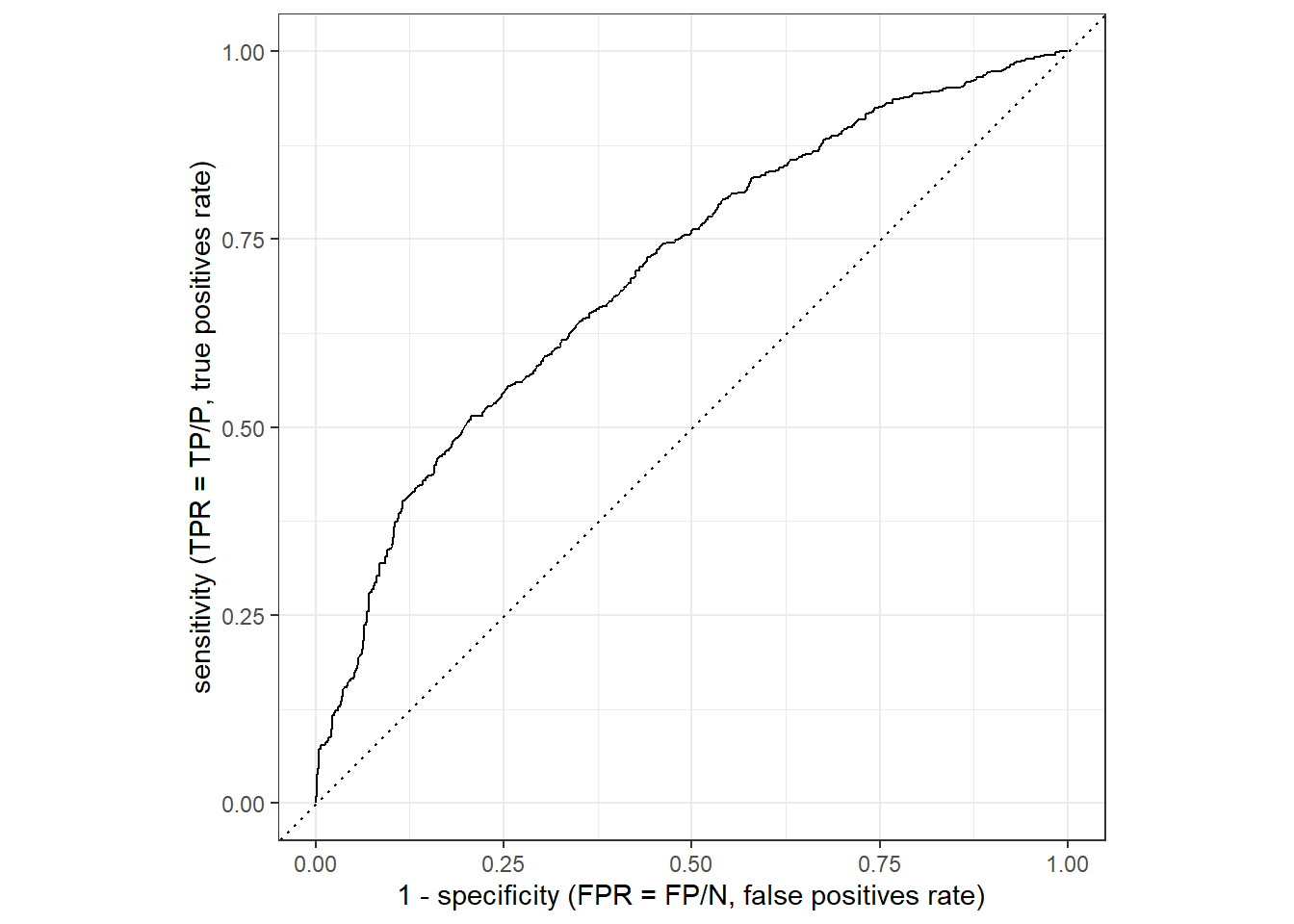

Figure 5: Precision, recall and threshold values

And we can also calculate the area under the ROC curve (the higher the better with 1 being the maximum as outlined here):

# Compute area under ROC curve
data_test %>% 
    roc_auc(truth = is_recid_factor, 
            .pred_yes,
              event_level = "second")

# A tibble: 1 × 3
  .metric .estimator .estimate
  <chr>   <chr>          <dbl>
1 roc_auc binary         0.706

Importantly, the ROC curve does not provide information on how FPR and TPR change as a function of the threshold. In Figure 6 we visualize both precision and recall (TPR) as a function of the threshold. The pr_curve() function can be used to calculate the corresponding values and we could also change it to FPR vs. TPR.

library(ggplot2)
library(dplyr)

data_test %>% 
  pr_curve(truth = is_recid_factor, 
           .pred_yes,
           event_level = "second") %>%
  pivot_longer(cols = c("recall", "precision"),
               names_to = "measure",
               values_to = "value") %>%
  mutate(measure = recode(measure,
                          "recall" = "Recall (= True pos. rate = TP/P = sensitivity)",
                          "precision" = "Precision (= Pos. pred. value = TP/P*)")) %>%
  ggplot(aes(x = .threshold, 
             y = value,
             color = measure)) +
  geom_line() +
  xlab("Threshold value") +
  ylab("Value of measure") +
  theme_bw()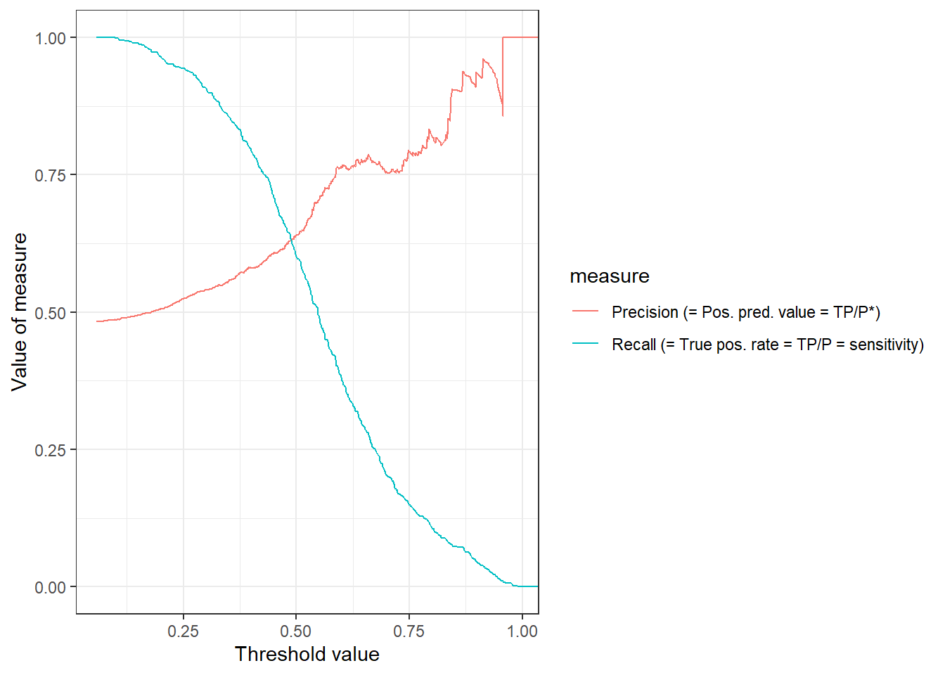

Figure 6: Precision, recall and threshold values

13 Exercise

Start by re-reading the code presented above (which you can find in the chunk below) to see whether everything is clear.
Above we re-evaluated the accuracy of our model using 10-fold cross validation. Please re-evaluate the model but now compare the setting where you use k-Fold Cross-Validation using 5 folds (k = 5) and 20 folds (k = 20). Do you find any differences?
Keep the same predictors but change the recipe and add polynomials for the numeric variables age, priors_count and use one_hot encoding for the race variable.² Does it change the accuracy?
Finally, shorty outline the advantages and disadvantages of the validation set approach (training/analyis vs. validation/assessment vs. test data), Leave-one-out cross-validation (LOOCV) and k-Fold Cross-Validation (e.g., discuss dataset sizes, representativeness, computational efficiency).

# install.packages(pacman)
pacman::p_load(tidyverse,
               tidymodels,
               knitr,
               kableExtra,
               DataExplorer,
               visdat,
               naniar)

rm(list=ls())
load(url(sprintf("https://docs.google.com/uc?id=%s&export=download",
                         "1gryEUVDd2qp9Gbgq8G0PDutK_YKKWWIk")))


# 1.
# Split the data into training and test data
  set.seed(345)
  data_split <- initial_split(data, prop = 0.8)
  data_split # Inspect

# Extract the two datasets
  data_train <- training(data_split)
  data_test <- testing(data_split) # Do not touch until the end!

# 2.  
# Create resampled partitions of training data
  data_folds <- vfold_cv(data_train, v = 10) # V-fold/k-fold cross-validation
  data_folds # data_folds now contains several resamples of our training data  
  # You can also try loo_cv(data_train) instead

  
  
# 3.
# Define the recipe & model
  recipe1 <- recipe(is_recid_factor ~ age + priors_count + 
                      sex + race, data = data_train) %>%
    step_poly(all_numeric_predictors(), degree = 4, 
              keep_original_cols = FALSE, 
              options = list(raw = TRUE)) %>% 
    step_dummy(race, one_hot = TRUE)
  
  model1 <- logistic_reg() %>% 
    set_engine("glm") %>% # lm engine
    set_mode("classification") # regression problem
  
# 4.
# Create workflow
  workflow1 <- 
  workflow() %>% 
  add_model(model1) %>%
  add_recipe(recipe1)

# 5. Fit the workflow on the folds/resamples
  # There is no need in specifying data_analysis/data_assessment as 
  # the functions understand the corresponding parts
  fit1 <- 
  workflow1 %>% 
  fit_resamples(resamples = data_folds,
                control = control_resamples(save_pred = TRUE,
                                            extract = function (x) extract_fit_parsnip(x)))
  fit1
  
# Extract single components from folds
  fit1$.metrics[1:2] # get first two rows of .metrics
  fit1$.extracts [1:2] # get first two rows of .extracts
  fit1$.extracts[[1]]$.extracts # Extract models

  
# 6. 
# Collect metrics across resamples
  collect_metrics(fit1)

# 7. 
  # Fit on training dataset (fit2!!!)
  fit2 <- workflow1 %>% fit(data = data_train)

  
# Training data: Add predictions & get metrics
  augment(fit2, data_train, type.predict = "response")  %>%
      metrics(truth = is_recid_factor, estimate = .pred_class)

  
  
# 8.   
# Test data: Add predictions & get metrics
  augment(fit2, data_test, type.predict = "response") %>%
      metrics(truth = is_recid_factor, estimate = .pred_class)
  
# More accuracy metrics
  metrics_combined <- metric_set(accuracy, precision, recall, f_meas)

  augment(fit2, data_test, type.predict = "response") %>%
  metrics_combined(truth = is_recid_factor, estimate = .pred_class)
  
# Cross-classification table
  augment(fit2, data_test, type.predict = "response") %>%
      conf_mat(data = .,
             truth = is_recid_factor, estimate = .pred_class)

Possible solutions

Rerun the code above but change settings in vfold_cv() to v = 5 and v = 10. Evaluate the metrics both in the test and training data.

# install.packages(pacman)
pacman::p_load(tidyverse,
               tidymodels,
               knitr,
               kableExtra,
               DataExplorer,
               visdat,
               naniar)

rm(list=ls())
load(url(sprintf("https://docs.google.com/uc?id=%s&export=download",
                         "1gryEUVDd2qp9Gbgq8G0PDutK_YKKWWIk")))


# 2. 
# Split the data into training and test data
  data_split <- initial_split(data, prop = 0.8)
  data_split # Inspect

# Extract the two datasets
  data_train <- training(data_split)
  data_test <- testing(data_split) # Do not touch until the end!

# Create resampled partitions of training data
  set.seed(345)
  data_folds <- vfold_cv(data_train, v =5) # V-fold/k-fold cross-validation
  data_folds # data_folds now contains several resamples of our training data  
  # You can also try loo_cv(data_train) instead

  
# Define the recipe & model
  recipe1 <- recipe(is_recid_factor ~ age + priors_count + 
                      sex + race, data = data_train)
  
  model1 <- logistic_reg() %>% 
    set_engine("glm") %>% # lm engine
    set_mode("classification") # regression problem
  
# Create workflow
  workflow1 <- 
  workflow() %>% 
  add_model(model1) %>%
  add_recipe(recipe1)

# Fit the workflow on the folds/resamples
  # There is no need in specifying data_analysis/data_assessment as 
  # the functions understand the corresponding parts
  fit1 <- 
  workflow1 %>% 
  fit_resamples(resamples = data_folds,
                control = control_resamples(save_pred = TRUE,
                                            extract = function (x) extract_fit_parsnip(x)))

# Collect metrics across resamples
  collect_metrics(fit1)

# Fit on training dataset (fit2!!!)
  fit2 <- workflow1 %>% fit(data = data_train)

# Training data: Add predictions 
  data_train <- augment(fit2, data_train, type.predict = "response") 

  head(data_train %>%
      select(is_recid_factor, age, .pred_class, .pred_no, .pred_yes))

# Training data: Metrics
  data_train %>%
      metrics(truth = is_recid_factor, estimate = .pred_class)

# Test data: Add predictions 
  data_test<- augment(fit2, data_test, type.predict = "response")

  head(data_test %>%
      select(is_recid_factor, age, .pred_class, .pred_no, .pred_yes))

# Test data: Metrics
  data_test %>%
      metrics(truth = is_recid_factor, estimate = .pred_class)
  
# More accuracy metrics
  metrics_combined <- metric_set(accuracy, precision, recall, f_meas)

  # The returned function has arguments:
  data_test %>% 
  metrics_combined(truth = is_recid_factor, estimate = .pred_class)
  
# Cross-classification table
  table(actual = data_test$is_recid_factor, predicted = data_test$.pred_class)

Advantages and disadvantages

Validation Set Approach (training vs. validation vs. test data)
- Advantages
  - Simple and easy to understand.
  - Faster than cross-validation methods due to a single split.
- Disadvantages
  - Results can vary significantly based on the data split.
  - Inefficient use of data, as a large portion is not used for training.
Leave-One-Out Cross-Validation (LOOCV)
- Advantages
  - Low bias as almost all data is used for training.
  - Every observation is used for both training and validation, ensuring a thorough assessment.
- Disadvantages
  - Computationally intensive for large datasets.
  - Can have high variance in performance estimates.
k-Fold Cross-Validation
- Advantages
  - Offers a balance between bias and variance.
  - Efficient use of data, with all observations used for both training and validation.
  - More computationally efficient than LOOCV.
- Disadvantages
  - The choice of (k) can affect performance estimates.
  - Variability in performance estimates due to randomness in splits.

14 Exercise: What’s predicted?

Q: What do we predict using the techniques below? What is the input/what is the output? How could we use those ML models for our own research? What phenomena may they create that we need to research? (discuss 2!)
1. Image recognition (Clarify) Image recognition (Google)
2. Speech recognition
3. Translation
4. Text analysis/Natural language processing (NLP)
5. Pose estimation (2018!)
6. Deepart [old link is dead link!]
7. Deep fakes (2019)

Insights

Image recognition: Predict whether an image shows a sunsetSome examples
Deepart: “Predict” what an image would look like if it was painted by…
Speech recognition: Predict which (written) words someone just used
Translation: Predict which English word/sentence corresponds to a German word/sentence (predict language!)
Pose estimation (2018!): Predict body pose from image
Deep fakes (2019): ?
Text analysis/Natural language processing (NLP): Predict entities, sentiment, syntax, categories in text

14.1 All the code

knitr::include_graphics("06_300px-LOOCV.gif")#
knitr::include_graphics("06_350px-KfoldCV.gif")#
# install.packages(pacman)
pacman::p_load(tidyverse,
               tidymodels,
               knitr,
               kableExtra,
               DataExplorer,
               visdat,
               naniar)
load(file = "www/data/data_compas.Rdata")
# install.packages(pacman)
pacman::p_load(tidyverse,
               tidymodels,
               knitr,
               kableExtra,
               DataExplorer,
               visdat,
               naniar)

rm(list=ls())
load(url(sprintf("https://docs.google.com/uc?id=%s&export=download",
                         "1gryEUVDd2qp9Gbgq8G0PDutK_YKKWWIk")))
# Extract data with missing outcome
  data_missing_outcome <- data %>% filter(is.na(is_recid_factor))
  dim(data_missing_outcome)

# Omit individuals with missing outcome from data
  data <- data %>% drop_na(is_recid_factor) # ?drop_na
  dim(data)


# 1.
# Split the data into training, validation and test data
  set.seed(1234)
  data_split <- initial_validation_split(data, prop = c(0.6, 0.2))
  data_split # Inspect

# Extract the datasets
  data_train <- training(data_split)
  data_validation <- validation(data_split)
  data_test <- testing(data_split) # Do not touch until the end!
  dim(data_train)
  dim(data_validation)
  dim(data_test)


# 2.
# Define the recipe & model
  recipe1 <- recipe(is_recid_factor ~ age + priors_count + 
                      sex + race, data = data_train)
  
  model1 <- logistic_reg() %>% 
    set_engine("glm") %>% # lm engine
    set_mode("classification") # regression problem
  
# 3.
# Create workflow
  workflow1 <- 
  workflow() %>% 
  add_model(model1) %>%
  add_recipe(recipe1)

# 4. Fit the workflow on training set & accuracy
  fit_train <- workflow1 %>% fit(data = data_train)

  data_train <- augment(fit_train, data_train, 
                        type.predict = "response") 

  data_train %>%
      metrics(truth = is_recid_factor, estimate = .pred_class)  
  

  # Predict & assess metrics in validation set
  augment(fit_train, data_validation, # Make sure to use training fit!
          type.predict = "response") %>%
      metrics(truth = is_recid_factor, estimate = .pred_class)    
  
  
# 5. If happy fit workflow on full 
  # training set (data_train + data validation) 
  # and predict values on test set
  data_training_full <- bind_rows(data_train, data_validation)
  fit_train_full <- workflow1 %>% fit(data = data_training_full)
  
  # Predict and assess accuracy
  augment(fit_train_full, data_test, 
          type.predict = "response") %>%
      metrics(truth = is_recid_factor, estimate = .pred_class)   
# install.packages(pacman)
pacman::p_load(tidyverse,
               tidymodels,
               knitr,
               kableExtra,
               DataExplorer,
               visdat,
               naniar)
load(file = "www/data/data_compas.Rdata")
# install.packages(pacman)
pacman::p_load(tidyverse,
               tidymodels,
               knitr,
               kableExtra,
               DataExplorer,
               visdat,
               naniar)

rm(list=ls())
load(url(sprintf("https://docs.google.com/uc?id=%s&export=download",
                         "1gryEUVDd2qp9Gbgq8G0PDutK_YKKWWIk")))
# Extract data with missing outcome
  data_missing_outcome <- data %>% 
                  filter(is.na(is_recid_factor))
  dim(data_missing_outcome)

# Omit individuals with missing outcome from data
  data <- data %>% drop_na(is_recid_factor) # ?drop_na
  dim(data)

# 1.
# Split the data into training and test data
  data_split <- initial_split(data, prop = 0.8)
  data_split # Inspect

# Extract the two datasets
  data_train <- training(data_split)
  data_test <- testing(data_split) # Do not touch until the end!

# 2.  
# Create resampled partitions of training data
  set.seed(345)
  data_folds <- vfold_cv(data_train, v = 10) # V-fold/k-fold cross-validation
  data_folds # data_folds now contains several resamples of our training data  
  # v = 10 -> n/10 gives number of validation set observation in each fold

  
  
# 3.
# Define the recipe & model
  recipe1 <- recipe(is_recid_factor ~ age + priors_count + 
                      sex + race, data = data_train)
  
  model1 <- logistic_reg() %>% 
    set_engine("glm") %>% # lm engine
    set_mode("classification") # regression problem
  
# 4.
# Create workflow
  workflow1 <- 
  workflow() %>% 
  add_model(model1) %>%
  add_recipe(recipe1)

# 5. Fit the workflow on the folds/resamples
  # There is no need in specifying 
  # data_analysis/data_assessment as 
  # the functions understand the corresponding parts
  fit1 <- 
  workflow1 %>% 
  fit_resamples(resamples = data_folds)
  # add argument "control" to keep predictions
    # control = control_resamples(save_pred = TRUE, extract = function (x) extract_fit_parsnip(x))
  
  fit1
  
# Extract single components from folds
  fit1$.metrics[1:2] # get first two rows of .metrics

  
# 6. 
# Collect metrics across resamples
  collect_metrics(fit1)
# 7. 
  # Fit on training dataset (fit2!!!)
  fit2 <- workflow1 %>% fit(data = data_train)

  
# Training data: Add predictions 
  data_train <- augment(fit2, data_train, type.predict = "response") 

  head(data_train %>%
      select(is_recid_factor, age, .pred_class, 
             .pred_no, .pred_yes))

# Training data: Metrics
  data_train %>%
      metrics(truth = is_recid_factor, estimate = .pred_class)
# 8. 
# Test data: Add predictions 
  data_test<- augment(fit2, data_test, type.predict = "response")

  head(data_test %>%
      select(is_recid_factor, age, .pred_class, .pred_no, .pred_yes))

# Test data: Metrics
  data_test %>%
      metrics(truth = is_recid_factor, estimate = .pred_class)
  
# More accuracy metrics
  metrics_combined <- metric_set(accuracy, precision, recall, f_meas)

  # The returned function has arguments:
  data_test %>% 
  metrics_combined(truth = is_recid_factor, estimate = .pred_class)
  
# Cross-classification table
  conf_mat(data = data_test,
           truth = is_recid_factor, estimate = .pred_class)

  
data_test %>% 
  roc_curve(truth = is_recid_factor, 
            .pred_yes,
            event_level = "second") %>% 
  autoplot() + 
  xlab("1 - specificity (FPR = FP/N, false positives rate)") +
  ylab("sensitivity (TPR = TP/P, true positives rate)")
# Compute area under ROC curve
data_test %>% 
    roc_auc(truth = is_recid_factor, 
            .pred_yes,
              event_level = "second")
library(ggplot2)
library(dplyr)

data_test %>% 
  pr_curve(truth = is_recid_factor, 
           .pred_yes,
           event_level = "second") %>%
  pivot_longer(cols = c("recall", "precision"),
               names_to = "measure",
               values_to = "value") %>%
  mutate(measure = recode(measure,
                          "recall" = "Recall (= True pos. rate = TP/P = sensitivity)",
                          "precision" = "Precision (= Pos. pred. value = TP/P*)")) %>%
  ggplot(aes(x = .threshold, 
             y = value,
             color = measure)) +
  geom_line() +
  xlab("Threshold value") +
  ylab("Value of measure") +
  theme_bw()
# install.packages(pacman)
pacman::p_load(tidyverse,
               tidymodels,
               knitr,
               kableExtra,
               DataExplorer,
               visdat,
               naniar)

rm(list=ls())
load(url(sprintf("https://docs.google.com/uc?id=%s&export=download",
                         "1gryEUVDd2qp9Gbgq8G0PDutK_YKKWWIk")))


# 1.
# Split the data into training and test data
  set.seed(345)
  data_split <- initial_split(data, prop = 0.8)
  data_split # Inspect

# Extract the two datasets
  data_train <- training(data_split)
  data_test <- testing(data_split) # Do not touch until the end!

# 2.  
# Create resampled partitions of training data
  data_folds <- vfold_cv(data_train, v = 10) # V-fold/k-fold cross-validation
  data_folds # data_folds now contains several resamples of our training data  
  # You can also try loo_cv(data_train) instead

  
  
# 3.
# Define the recipe & model
  recipe1 <- recipe(is_recid_factor ~ age + priors_count + 
                      sex + race, data = data_train) %>%
    step_poly(all_numeric_predictors(), degree = 4, 
              keep_original_cols = FALSE, 
              options = list(raw = TRUE)) %>% 
    step_dummy(race, one_hot = TRUE)
  
  model1 <- logistic_reg() %>% 
    set_engine("glm") %>% # lm engine
    set_mode("classification") # regression problem
  
# 4.
# Create workflow
  workflow1 <- 
  workflow() %>% 
  add_model(model1) %>%
  add_recipe(recipe1)

# 5. Fit the workflow on the folds/resamples
  # There is no need in specifying data_analysis/data_assessment as 
  # the functions understand the corresponding parts
  fit1 <- 
  workflow1 %>% 
  fit_resamples(resamples = data_folds,
                control = control_resamples(save_pred = TRUE,
                                            extract = function (x) extract_fit_parsnip(x)))
  fit1
  
# Extract single components from folds
  fit1$.metrics[1:2] # get first two rows of .metrics
  fit1$.extracts [1:2] # get first two rows of .extracts
  fit1$.extracts[[1]]$.extracts # Extract models

  
# 6. 
# Collect metrics across resamples
  collect_metrics(fit1)

# 7. 
  # Fit on training dataset (fit2!!!)
  fit2 <- workflow1 %>% fit(data = data_train)

  
# Training data: Add predictions & get metrics
  augment(fit2, data_train, type.predict = "response")  %>%
      metrics(truth = is_recid_factor, estimate = .pred_class)

  
  
# 8.   
# Test data: Add predictions & get metrics
  augment(fit2, data_test, type.predict = "response") %>%
      metrics(truth = is_recid_factor, estimate = .pred_class)
  
# More accuracy metrics
  metrics_combined <- metric_set(accuracy, precision, recall, f_meas)

  augment(fit2, data_test, type.predict = "response") %>%
  metrics_combined(truth = is_recid_factor, estimate = .pred_class)
  
# Cross-classification table
  augment(fit2, data_test, type.predict = "response") %>%
      conf_mat(data = .,
             truth = is_recid_factor, estimate = .pred_class)
           
  
# install.packages(pacman)
pacman::p_load(tidyverse,
               tidymodels,
               knitr,
               kableExtra,
               DataExplorer,
               visdat,
               naniar)

rm(list=ls())
load(url(sprintf("https://docs.google.com/uc?id=%s&export=download",
                         "1gryEUVDd2qp9Gbgq8G0PDutK_YKKWWIk")))


# 2. 
# Split the data into training and test data
  data_split <- initial_split(data, prop = 0.8)
  data_split # Inspect

# Extract the two datasets
  data_train <- training(data_split)
  data_test <- testing(data_split) # Do not touch until the end!

# Create resampled partitions of training data
  set.seed(345)
  data_folds <- vfold_cv(data_train, v =5) # V-fold/k-fold cross-validation
  data_folds # data_folds now contains several resamples of our training data  
  # You can also try loo_cv(data_train) instead

  
# Define the recipe & model
  recipe1 <- recipe(is_recid_factor ~ age + priors_count + 
                      sex + race, data = data_train)
  
  model1 <- logistic_reg() %>% 
    set_engine("glm") %>% # lm engine
    set_mode("classification") # regression problem
  
# Create workflow
  workflow1 <- 
  workflow() %>% 
  add_model(model1) %>%
  add_recipe(recipe1)

# Fit the workflow on the folds/resamples
  # There is no need in specifying data_analysis/data_assessment as 
  # the functions understand the corresponding parts
  fit1 <- 
  workflow1 %>% 
  fit_resamples(resamples = data_folds,
                control = control_resamples(save_pred = TRUE,
                                            extract = function (x) extract_fit_parsnip(x)))

# Collect metrics across resamples
  collect_metrics(fit1)

# Fit on training dataset (fit2!!!)
  fit2 <- workflow1 %>% fit(data = data_train)

# Training data: Add predictions 
  data_train <- augment(fit2, data_train, type.predict = "response") 

  head(data_train %>%
      select(is_recid_factor, age, .pred_class, .pred_no, .pred_yes))

# Training data: Metrics
  data_train %>%
      metrics(truth = is_recid_factor, estimate = .pred_class)

# Test data: Add predictions 
  data_test<- augment(fit2, data_test, type.predict = "response")

  head(data_test %>%
      select(is_recid_factor, age, .pred_class, .pred_no, .pred_yes))

# Test data: Metrics
  data_test %>%
      metrics(truth = is_recid_factor, estimate = .pred_class)
  
# More accuracy metrics
  metrics_combined <- metric_set(accuracy, precision, recall, f_meas)

  # The returned function has arguments:
  data_test %>% 
  metrics_combined(truth = is_recid_factor, estimate = .pred_class)
  
# Cross-classification table
  table(actual = data_test$is_recid_factor, predicted = data_test$.pred_class)

  
labs = knitr::all_labels()
ignore_chunks <- labs[str_detect(labs, "exclude|setup|solution|get-labels")]
labs = setdiff(labs, ignore_chunks)

References

James, Gareth, Daniela Witten, Trevor Hastie, and Robert Tibshirani. 2013. An Introduction to Statistical Learning: With Applications in R. Springer Texts in Statistics. Springer.

Neunhoeffer, Marcel, and Sebastian Sternberg. 2019. “How Cross-Validation Can Go Wrong and What to Do about It.” Polit. Anal. 27 (1): 101–6.

Footnotes

Tip: ChatGPT prompt -> What is a very simple example of the variance inflation phenomenon?↩︎
step_poly(all_numeric_predictors(), degree = 4, keep_original_cols = TRUE, options = list(raw = TRUE)) %>% step_dummy(race, one_hot = TRUE)↩︎