Bias and fairness of ML models
Learning outcomes/objective: Learn…
- …about the discussion surrounding bias/fairness in machine learning and the underlying concepts.
- …how to assess whether an algorithm is biased.
- …how to assess algorithmic bias in R.
Sources: Mehrabi et al. (2021), Dressel and Farid (2018), Osoba and Welser (2017), Lee, Du, and Guerzhoy (2020)
1 Overview
- ‘like people, algorithms are vulnerable to biases that render their decisions “unfair”’ (Mehrabi et al. 2021, 115:2)
- Decision-making context: “fairness is the absence of any prejudice or favoritism toward an individual or group based on their inherent or acquired characteristics” (Mehrabi et al. 2021, 115:2)
- Example: Correctional Offender Management Profiling for Alternative Sanctions (COMPAS)
- Measures the risk of a person to recommit another crime
- Judges use COMPAS to decide whether to release an offender or to keep him or her in prison
- “COMPAS is more likely to have higher false positive rates for African-American offenders than Caucasian offenders in falsely predicting them to be at a higher risk of recommitting a crime or recidivism” (Mehrabi et al. 2021, 115:2)
- Sources of bias can be biases in the data and biases in the algorithms
- Assessment tools: Aequitas; Bias and Fairness Audit Toolkit (Microsoft Fair Learn); The What-if Tool (Google) IBM 360 degree toolkit
- Research: e.g., projects such as Trustworthiness Auditing for AI
- …unfair predictions based on unfair data
2 Biases in a feed-back loop
- Figure 1 visualizes the loop capturing the feedback between biases in data, algorithms, and user interaction.
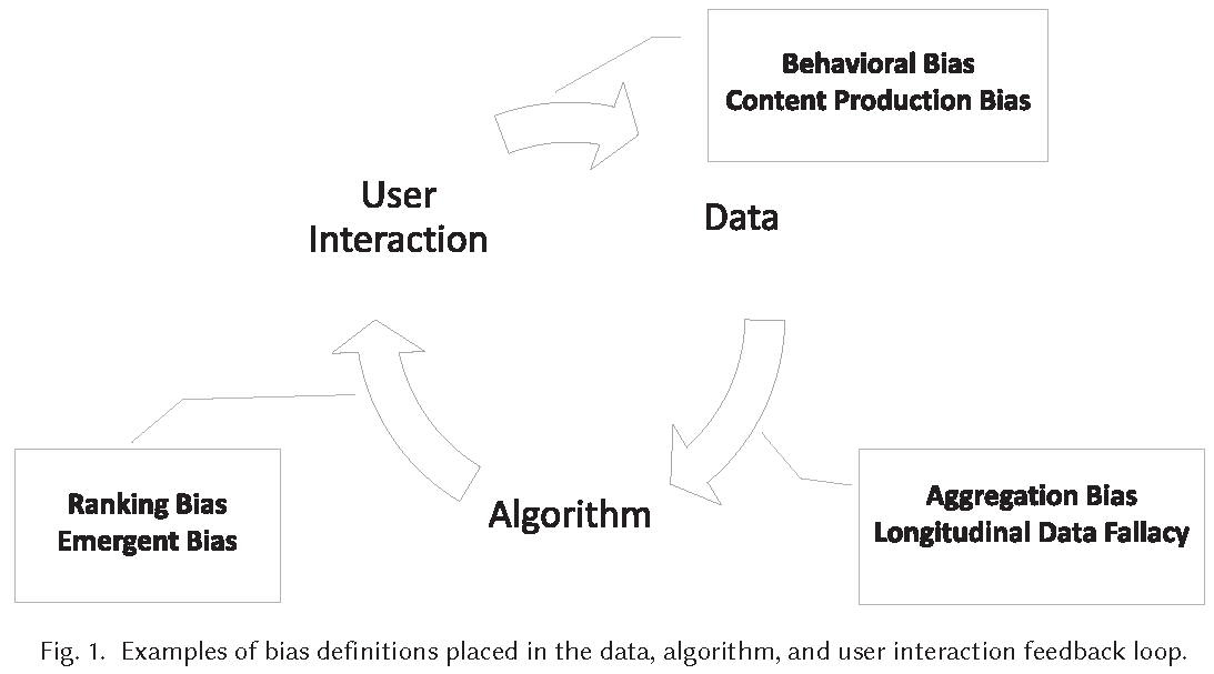
- Biases in data feed into algorithms that affect user interaction that feeds into data
- Example of web search engine (Mehrabi et al. 2021, 115:4)
- Algorithm: Puts specific results at the top of its list and users tend to interact most with the top results
- User interaction: Interactions of users with items will then be collected by web search engine, and data will be used to make future decisions on how information should be presented based on popularity and user interest
- Data: Results at the top will become more and more popular, not because of the nature of the result but due to the biased interaction and placement of results by these algorithms
- Q: Can you think of other examples?
3 Exercise: Biases in a feed-back loop
- Q: Discuss with your neighbor on how/wether this feedback loop in Figure 2 exists in the case of the recidivism example.
4 Types of bias
- Source: Mehrabi et al. (2021, sec. 3.1)
4.1 Biases: Data to Algoritm
- Measurement Bias: arises from how we choose, utilize, and measure particular features
- e.g., COMPAS, where prior arrests and friend/family arrests were used as proxy variables to measure level of “riskiness” or “crime”
- Omitted Variable Bias: occurs when one or more important variables [predictors] are left out of the model1
- Representation Bias: arises from how we sample from a population during data collection process
- e.g. ImageNet: bias towards Western cultures (see Figure 3 and 4 in Mehrabi et al. 2021)
- Aggregation Bias (or ecological fallacy): arises when false conclusions are drawn about individuals from observing the entire population
- Sampling Bias: is similar to representation bias, and arises due to non-random sampling of subgroups
- Longitudinal Data Fallacy: Researchers analyzing temporal data must use longitudinal analysis to track cohorts over time to learn their behavior. Instead, temporal data is often modeled using cross-sectional analysis, which combines diverse cohorts at a single time point4
- Linking Bias: arises when network attributes obtained from user connections, activities, or interactions differ and misrepresent the true behavior of the users5
- Q: Can you think of concrete examples of how data biases may feed into algorithms?
4.2 Biases: Algorithm to User
- Algorithmic Bias: bias is not present in the input data but purely produced by the algorithm
- Originates from design/modelling choices: optimization functions, regularizations, choices in applying regression models on the data as a whole or considering subgroups, and the general use of statistically biased estimators in algorithms
- User Interaction Bias: type of bias that can not only be observant on the Web but also get triggered from two sources—the user interface and through the user itself by imposing his/her self-selected biased behavior and interaction (e.g., Presentation Bias6, Ranking Bias7)
- Popularity Bias: Items that are more popular tend to be exposed more. However, popularity metrics are subject to manipulation—for example, by fake reviews or social bots
- Emergent Bias: occurs as a result of use and interaction with real users. This bias arises as a result of change in population, cultural values, or societal knowledge (e.g., different people use same interface differently; Q: Example?)
- Evaluation Bias: Evaluation bias happens during model evaluation8
- Q: Can you think of concrete examples of how algorithm biases may feed into user interaction?
4.3 Biases: User to Data
User-induced biases through user-generated data (e.g., humans flagging facebook content)
Historical Bias: Already existing bias and socio-technical issues in the world and can seep into ML model from the data generation process even given a perfect sampling and feature selection
- e.g., 2018 image search result where searching for women CEOs ultimately resulted in fewer female CEO images due to the fact that only 5% of Fortune 500 CEOs were women—which would cause the search results to be biased towards male CEOs (reflects reality but do we want that)
Population Bias: arises when statistics, demographics, representatives, and user characteristics are different in the user population of the platform from the original target population (e.g., populations across platforms vary)
Self-selection Bias: is a subtype of the selection or sampling bias in which subjects of the research select themselves
- e.g., enthusiastic supporters of candidate are more likely to complete the poll that should measure popularity of their candidate.
Social Bias: happens when others’ actions affect our judgment
- e.g., we want to rate or review an item with a low score, but are influenced by other high ratings (Q: Can you think of an example?)
Behavioral Bias: arises from different user behavior across platforms, contexts, or different datasets
- e.g., differences in emoji representations among platforms can result in different reactions and behavior from people and sometimes even leading to communication errors
Temporal Bias: arises from differences in populations and behaviors over time
- e.g., Twitter where people talking about a particular topic start using a hashtag at some point to capture attention, then continue the discussion about the event without using the hashtag
Content Production Bias: Content Production bias arises from structural, lexical, semantic, and syntactic differences in the contents generated by users
- e.g., differences in use of language across different gender and age groups
4.4 Discrimination (1)
- Discrimination: “a source for unfairness that is due to human prejudice and stereotyping based on the sensitive attributes, which may happen intentionally or unintentionally” (Mehrabi et al. 2021, 115:10)
- “while bias can be considered as a source for unfairness that is due to the data collection, sampling, and measurement” (Mehrabi et al. 2021, 115:10)
- Explainable Discrimination: Differences in treatment and outcomes among different groups can be justified and explained via some attributes and are not considered illegal as a consequence
- UCI Adult dataset (Kamiran and Žliobaitė 2013): Dataset used in fairness domain where males on average have a higher annual income than females
- Reason: On average females work fewer hours than males per week
- UCI Adult dataset (Kamiran and Žliobaitė 2013): Dataset used in fairness domain where males on average have a higher annual income than females
- Q: What do you think is reverse discrimination?
- Q: Can you give other examples of explainable discrimination?
4.5 Discrimination (2)
- Unexplainable Discrimination: Unexplainable discrimination in which the discrimination toward a group is unjustified and therefore considered illegal
- Direct discrimination: happens when protected attributes of individuals explicitly result in non-favorable outcomes toward them (e.g., race, sex, etc.)
- see Table 3 (Mehrabi et al. 2021, 115:15)
- Indirect discrimination: individuals appear to be treated based on seemingly neutral and non-protected attributes; however, protected groups, or individuals, still get to be treated unjustly as a result of implicit effects from their protected attributes (e.g., residential zip code: Q:why?)
- Q: Can you think of other examples of indirect discrimination?
- Direct discrimination: happens when protected attributes of individuals explicitly result in non-favorable outcomes toward them (e.g., race, sex, etc.)
- Sources of discrimination
- Systemic discrimination: refers to policies, customs, or behaviors that are a part of the culture or structure of an organization that may perpetuate discrimination against certain subgroups of the population
- Statistical discrimination: a phenomenon where decision-makers use average group statistics to judge an individual belonging to that group
5 Algorithmic fairness (1)
- No universal definition of fairness (Saxena 2019)
- Fairness: “absence of any prejudice or favoritism towards an individual or a group based on their intrinsic or acquired traits in the context of decision-making” (Saxena et al. 2019)
- Many different definitions of fairness (Mehrabi et al. 2021; Verma and Rubin 2018)
- Definition 1 (Equalized Odds) (Hardt, Price, and Srebro 2016): probability of a person in the positive class being correctly assigned a positive outcome and the probability of a person in a negative class being incorrectly assigned a positive outcome should both be the same for the protected and unprotected group members (Verma and Rubin 2018), i.e, protected and unprotected groups should have equal rates for true positives and false positives
- Definition 2 (Equal Opportunity) (Hardt, Price, and Srebro 2016): probability of a person in a positive class being assigned to a positive outcome should be equal for both protected and unprotected (female and male) group members (Verma and Rubin 2018), i.e., the equal opportunity definition states that the protected and unprotected groups should have equal true positive rates
More definitions of fairness
See discussions in Mehrabi et al. (2021) and Verma and Rubin (2018).
Definition 3 (Demographic Parity) (Dwork et al. 2012; Kusner et al. 2017): also known as statistical parity …the likelihood of a positive outcome should be the same regardless of whether the person is in the protected (e.g., female) group (Verma and Rubin 2018)
Definition 4 (Fairness through Awareness): “An algorithm is fair if it gives similar predictions to similar individuals” (Dwork et al. 2012; Kusner et al. 2017), i.e., two individuals who are similar with respect to a similarity (inverse distance) metric defined for a particular task should receive a similar outcome.
Definition 5 (Fairness through Unawareness) : “An algorithm is fair as long as any protected attributes A are not explicitly used in the decision-making process” Kusner et al. (2017)
Definition 6 (Treatment Equality): “Treatment equality is achieved when the ratio of false negatives and false positives is the same for both protected group categories” (Berk et al. 2021).
…to be continued (cf. Mehrabi et al. 2021, sec. 4).
6 Algorithmic fairness (2)
- Fairness definitions fall into different types as shown in Table in Figure 3.
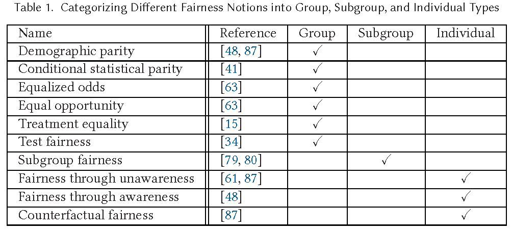
- (1) Individual Fairness: Give similar predictions to similar individuals
- (2) Group Fairness: Treat different groups equally
- (3) Subgroup Fairness:
- Subgroup fairness intends to obtain the best properties of the group and individual notions of fairness. It is different than these notions but uses them to obtain better outcomes.
- It picks a group fairness constraint like equalizing false positive and asks whether this constraint holds over a large collection of subgroups
7 Retake: Accuracy & false positives & negatives
- Accuracy = Correct Classification Rate (CCR) = 1 - Error Rate
- For what proportion of the units does the correct output \(y_{i}\) match the classifier (predicted) output \(\hat{y}_{i}\)?
- Proportion of reoffenders correctly predicted
- See Figure 5
- \((TN + TP)/(TN + TP + FN + FP)\)
- False Positive Rate (FPR)
- What then is the False Negative Rate (FNR) in Figure 5?

8 Fairness assessment
- Algorithmic fairness can be assessed with respect to an input characteristic \(C\), e.g., race, sex
- False positive parity…
- …is satisfied with respect to characteristic \(C\) if false positive rate (\(FPR=FP/N\)) for inputs with \(C = 0\) (e.g., black) is same as false positive rate for inputs with \(C = 1\) (e.g., white)
- ProPublica found that the false positive rate for African-American defendants (i.e., the percentage of innocent African-American defendants classified as likely to re-offend) was higher than for white defendants (→ NO false positive parity)
- Calibration…
- …satisfied with respect to characteristic \(C\) if individuals who were labeled “positive” have the same probability of actually being positive, regardless of the value of \(C\)…
- …and if individuals who were labeled “negative” have the same probability of actually being negative regardless of the value of \(C\)
- COMPAS makers claim that COMPAS satisfies calibration!
9 Tidymodels: Fairness assessment
- Key Functions
metric_set(accuracy, precision, recall, f_meas, npv, spec, sens, ppv): Define metric set the includes all sorts of metricsmetrics_combined <- metric_set(): Assign metric set to object so it can be applied to data- Metrics
accuracy(): Proportion of correctly predicted cases (true/actual = predicted) among total cases - \((TN + TP)/(TN + TP + FN + FP)\)precision()orppv(): Proportion of actual positives (= 1) among positive predictions - \((TP/P*= \text{Positive predictive value})\)recall()orsens(): Proportion of actual positives (= 1) correctly identified - \((TP/P = \text{True positive rate})\)spec()ornpv(): proportion of actual/true negatives (= 0) correctly identified - \((TN/N*= \text{Specificity/Negative predictive value})\)1 - spec(): Proportion of actual positives (= 1) correctly identified (False Positive Rate) - \((FP/N = \text{False positive rate})\)- Not include in
yardstick…
- Not include in
f_meas(): Harmonic mean of precision and recall
Confusion matrix for retake
10 Lab: Assessing algorithmic fairness in R
See here for a description of the data and illustration of how to explore the data. Below we explore how to assess algorithmic fairness for the variable race.
Overview of Compas dataset variables
id: ID of prisoner, numericname: Name of prisoner, factorcompas_screening_date: Date of compass screening, datedecile_score: the decile of the COMPAS score, numericis_recid: whether somone reoffended/recidivated (=1) or not (=0), numericis_recid_factor: same but factor variableage: a continuous variable containing the age (in years) of the person, numericage_cat: age categorizedpriors_count: number of prior crimes committed, numericsex: gender with levels “Female” and “Male”, factorrace: race of the person, factorjuv_fel_count: number of juvenile felonies, numericjuv_misd_count: number of juvenile misdemeanors, numericjuv_other_count: number of prior juvenile convictions that are not considered either felonies or misdemeanors, numeric
We first import the data into R:
Explore and visualize the race variable.
Q: What do we find?
| Race | Frequency |
|---|---|
| African-American | 3696 |
| Asian | 32 |
| Caucasian | 2454 |
| Hispanic | 637 |
| Native American | 18 |
| Other | 377 |
| NA | 0 |
data %>%
ggplot(aes(x = fct_infreq(race))) + # fct_infreq(): reoder according to frequency
geom_bar() + # create barplot
geom_text(stat = "count", # add proportions
aes(label = round((after_stat(count)) / sum(after_stat(count)), 2),
vjust = -0.5))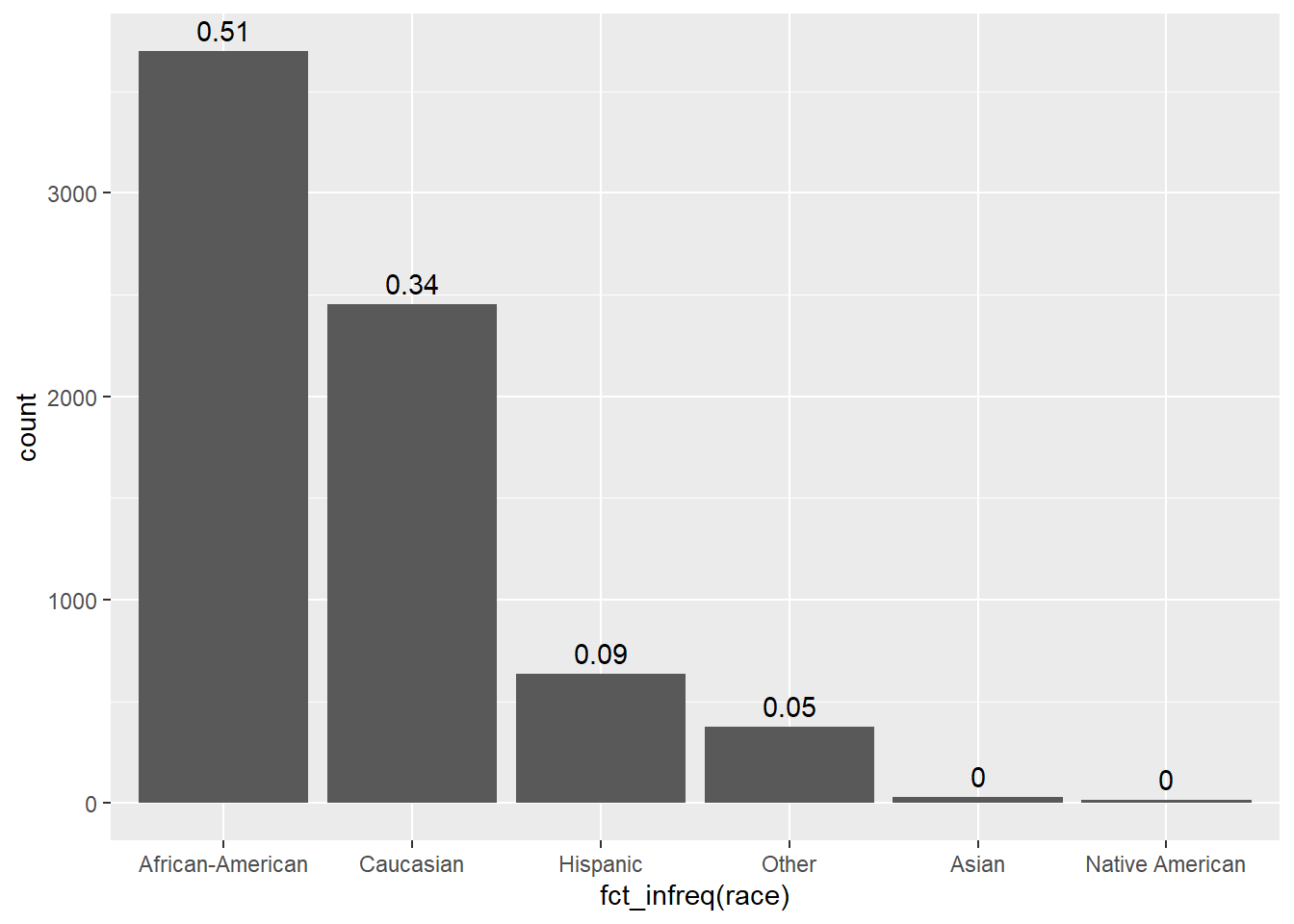
10.1 Estimate model
Below we estimate the MLM that we want to evaluate later on (using a workflow and without resampling).
# Extract data with missing outcome
data_missing_outcome <- data %>% filter(is.na(is_recid_factor))
dim(data_missing_outcome)[1] 614 14# Omit individuals with missing outcome from data
data <- data %>% drop_na(is_recid_factor) # ?drop_na
dim(data)[1] 6600 14# Split the data into training and test data
data_split <- initial_split(data, prop = 0.80)
data_split # Inspect<Training/Testing/Total>
<5280/1320/6600># Extract the two datasets
data_train <- training(data_split)
data_test <- testing(data_split) # Do not touch until the end!
# Define a recipe for preprocessing (taken from above)
recipe1 <- recipe(is_recid_factor ~ age + priors_count + race, data = data_train) %>%
step_normalize(all_numeric_predictors()) %>%
step_poly(all_numeric_predictors(), degree = 3) # Increase flexibility/parameters
# Define a model
model1 <- logistic_reg() %>% # logistic model
set_engine("glm") %>% # define lm package/function
set_mode("classification")
# Define a workflow
workflow1 <- workflow() %>% # create empty workflow
add_recipe(recipe1) %>% # add recipe
add_model(model1) # add model
# Fit the workflow (including recipe and model)
fit1 <- workflow1 %>% fit(data = data_train)
# Define metrics
metrics_combined <- metric_set(accuracy, precision, recall, f_meas,
spec)
# Training data: Add predictions & accuracy
data_train <- augment(fit1, data_train, type.predict = "response")
data_train_metrics <- data_train %>%
select(is_recid_factor, age, .pred_class, .pred_no, .pred_yes) %>%
metrics_combined(truth = is_recid_factor, estimate = .pred_class)
# Add FPR
data_train_metrics <- data_train_metrics %>%
add_row(.metric = "FPR", .estimator="binary", .estimate = 1-.$.estimate[5])
# Explain logic -> .$.estimate[5]
data_train_metrics# A tibble: 6 × 3
.metric .estimator .estimate
<chr> <chr> <dbl>
1 accuracy binary 0.673
2 precision binary 0.680
3 recall binary 0.674
4 f_meas binary 0.677
5 spec binary 0.672
6 FPR binary 0.328# Test data: Add predictions & accuracy
data_test <- augment(fit1, data_test, type.predict = "response")
data_test_metrics <- data_test %>%
select(is_recid_factor, age, .pred_class, .pred_no, .pred_yes) %>%
metrics_combined(truth = is_recid_factor, estimate = .pred_class)
# Add FPR
data_test_metrics <- data_test_metrics %>%
add_row(.metric = "FPR", .estimator="binary", .estimate = 1-.$.estimate[5])
data_test_metrics# A tibble: 6 × 3
.metric .estimator .estimate
<chr> <chr> <dbl>
1 accuracy binary 0.687
2 precision binary 0.735
3 recall binary 0.690
4 f_meas binary 0.712
5 spec binary 0.683
6 FPR binary 0.317Subsequently, we can use the obtained datasets that include the predictions to explore algorithmic bias.
10.2 Fairness evaluation: Functions
Here, we are computing the False Positive Rate (FPR), False Negative Rate (FNR) and the correct classification rate (CCR) for different populations.To do so we use the test data data_test. First, we’ll define functions get_FPR, get_FNR and get_CCR to compute the false positive rate (FPR), the false negative rate (FNR) and the correct classification rate (CCR). Below we describe the arguments in those functions:
data_setargument is used to define the dataset, i.e., we can calculate these rates indata_analysis,data_testordata_test.thrargument in the functions is used to define the threshold (usually \(0.5\))outcomeargument will contain the outcome variableis_recid_factorwhich is the actual outcome variableprobability_predictedargument is used to define the predicted probability
# Function: False Positive Rate
get_FPR <- function(data_set, # Use assessment or test data here
outcome, # Specify outcome variable
probability_predicted, # Specify var containting pred. probs.
thr) { # Specify threshold
return( # display results
# Sum above threshold AND NOT recidivate
sum((data_set %>% select(dplyr::all_of(probability_predicted)) >= thr) &
(data_set %>% select(dplyr::all_of(outcome)) == 0), na.rm = TRUE)
/ # divided by
# Sum NOT recividate
sum(data_set %>% select(dplyr::all_of(outcome)) == 0, na.rm = TRUE)
)
}
# Share of people over the threshold that did not recidivate
# of all that did not recidivate (who got falsely predicted to
# recidivate)
# Q: Please explain the function below!
# Function: False Negative Rate
get_FNR <- function(data_set,
outcome,
probability_predicted,
thr) {
return(
sum((data_set %>% select(dplyr::all_of(probability_predicted)) < thr) &
(data_set %>% select(dplyr::all_of(outcome)) == 1), na.rm = TRUE) # ?
/
sum(data_set %>% select(dplyr::all_of(outcome)) == 1, na.rm = TRUE)
) # ?
}
# Q: Explain the function below!
# Function: Correct Classification Rate
get_CCR <- function(data_set,
outcome,
probability_predicted,
thr) {
return(
mean((data_set %>% select(dplyr::all_of(probability_predicted)) >= thr) # ?
==
data_set %>% select(dplyr::all_of(outcome)), na.rm = TRUE)
) # ?
}We start by creating a nested dataframe data_test_groups that contains dataframes of data_test for all observations and subsets thereof (ethnic groups).
data_test_all <- data_test %>%
mutate(race = "All") %>% # replace grouping variable with constant
nest(.by = "race")
data_test_groups_race <- data_test %>%
nest(.by = "race")
data_test_groups <- bind_rows(
data_test_all,
data_test_groups_race
)
data_test_groups# A tibble: 7 × 2
race data
<chr> <list>
1 All <tibble [1,320 × 16]>
2 African-American <tibble [676 × 16]>
3 Caucasian <tibble [442 × 16]>
4 Hispanic <tibble [128 × 16]>
5 Other <tibble [65 × 16]>
6 Native American <tibble [5 × 16]>
7 Asian <tibble [4 × 16]> 10.3 Fairness evaluation: COMPAS scores
Then we apply our functions to data_test_groups with thr = \(5\) because COMPAS score decile_score, our predicted probability, goes from 0-10 instead of 0-1.
data_test_groups %>%
mutate(
FPR = map_dbl(
.x = data, # Nested column that includes the datasets
~ get_FPR( # Function to get FPR
data_set = .x,
outcome = "is_recid",
probability_predicted = "decile_score",
thr = 5
)
),
FNR = map_dbl(
.x = data,
~ get_FNR(
data_set = .x,
outcome = "is_recid",
probability_predicted = "decile_score",
thr = 5
)
),
CCR = map_dbl(
.x = data,
~ get_CCR(
data_set = .x,
outcome = "is_recid",
probability_predicted = "decile_score",
thr = 5
)
)
) %>%
mutate_if(is.numeric, round, digits = 2)# A tibble: 7 × 5
race data FPR FNR CCR
<chr> <list> <dbl> <dbl> <dbl>
1 All <tibble [1,320 × 16]> 0.34 0.38 0.64
2 African-American <tibble [676 × 16]> 0.46 0.29 0.62
3 Caucasian <tibble [442 × 16]> 0.26 0.46 0.67
4 Hispanic <tibble [128 × 16]> 0.23 0.67 0.61
5 Other <tibble [65 × 16]> 0.14 0.68 0.68
6 Native American <tibble [5 × 16]> 0.33 0 0.8
7 Asian <tibble [4 × 16]> 0 0.5 0.75We can see that the COMPAS score decile_score do not satisfy false positive parity and do not satisfy false negative parity. The scores do satisfy classification parity. Demographic parity is also not satisfied.
10.4 Fairness evaluation: Our model
Let’s now obtain the FPR, FNR, and CCR for our own predictive logistic regression model, using the threshold \(0.5\). We use the dataset from above that includes the predictios in .pred_ye. Importantly, we have to use the numeric version of our outcome variable is_recid (that’s how the function is written). Then we basically do the same as above, however, now we don’t use the COMPAS scores stored in decile_score but use our own predicted values stored in the variable prediction. The predicted values are between 0 and 1 and not deciles as in decile_score. Hence, we have to change thr from \(5\) to \(0.5\).
data_test_groups <-
data_test_groups %>%
mutate(
FPR = map_dbl(
.x = data,
~ get_FPR(
data_set = .x,
outcome = "is_recid",
probability_predicted = ".pred_yes",
thr = 0.5
)
),
FNR = map_dbl(
.x = data,
~ get_FNR(
data_set = .x,
outcome = "is_recid",
probability_predicted = ".pred_yes",
thr = 0.5
)
),
CCR = map_dbl(
.x = data,
~ get_CCR(
data_set = .x,
outcome = "is_recid",
probability_predicted = ".pred_yes",
thr = 0.5
)
)
) %>%
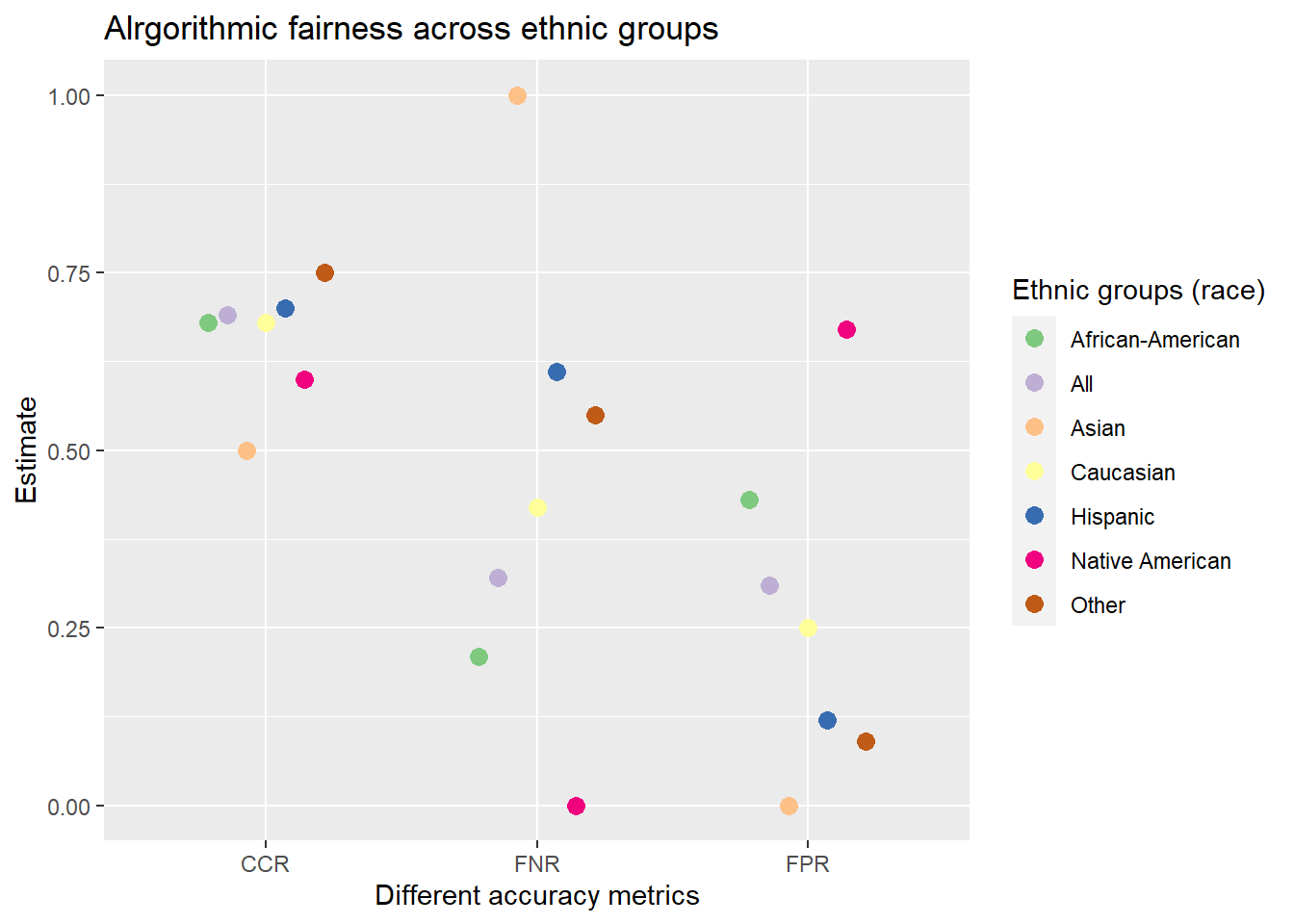
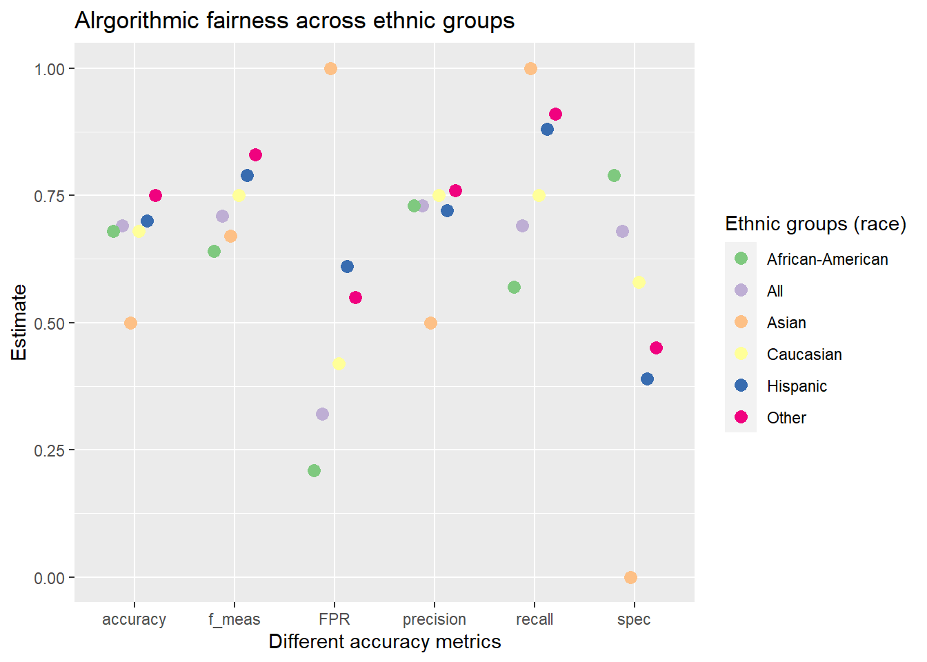
mutate_if(is.numeric, round, digits = 2)We can see that the FPR is higher for African-Americans as compared to Caucasians (the FNR is lower). Hence, they are treated unfairly.
And we can visualize those results:
# Pivtot the metric results into longformat
data_plot <- data_test_groups %>%
select(race, FPR, FNR, CCR) %>%
pivot_longer(cols = c("FPR", "FNR", "CCR"),
names_to = "Metric",
values_to = "Estimate")
data_plot %>%
ggplot(mapping = aes(
x = Metric,
y = Estimate,
color = race
)) +
geom_point(size = 3, position=position_dodge(width = .5)) +
scale_color_brewer(type ="qual") +
labs(
title = "Alrgorithmic fairness across ethnic groups",
x = "Different accuracy metrics",
y = "Estimate",
color = "Ethnic groups (race)"
)
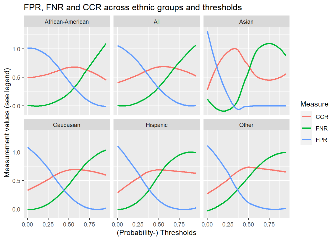
10.5 Altering the threshold (of our model!)
We can also explore how changing the threshold influences the false positive, false negative, and correct classification rates for the different ethnic groups. Below we use a combination of expand(), nesting() and map() with our functions to produce and visualize the corresponding data. You can execute the code step by step (from pipe to pipe).
[1] 0.00 0.01 0.02 0.03 0.04 0.05 0.06 0.07 0.08 0.09 0.10 0.11 0.12 0.13 0.14
[16] 0.15 0.16 0.17 0.18 0.19 0.20 0.21 0.22 0.23 0.24 0.25 0.26 0.27 0.28 0.29
[31] 0.30 0.31 0.32 0.33 0.34 0.35 0.36 0.37 0.38 0.39 0.40 0.41 0.42 0.43 0.44
[46] 0.45 0.46 0.47 0.48 0.49 0.50 0.51 0.52 0.53 0.54 0.55 0.56 0.57 0.58 0.59
[61] 0.60 0.61 0.62 0.63 0.64 0.65 0.66 0.67 0.68 0.69 0.70 0.71 0.72 0.73 0.74
[76] 0.75 0.76 0.77 0.78 0.79 0.80 0.81 0.82 0.83 0.84 0.85 0.86 0.87 0.88 0.89
[91] 0.90 0.91 0.92 0.93 0.94 0.95# Expand df with threshold values and calculate rates
data_test_groups %>%
filter(race != "Native American") %>% # too few observations
expand(nesting(race, data), thrs) %>%
mutate(
FPR = map2_dbl(
.x = data,
.y = thrs,
~ get_FPR(
data_set = .x,
outcome = "is_recid",
probability_predicted = ".pred_yes",
thr = .y
)
),
FNR = map2_dbl(
.x = data,
.y = thrs,
~ get_FNR(
data_set = .x,
outcome = "is_recid",
probability_predicted = ".pred_yes",
thr = .y
)
),
CCR = map2_dbl(
.x = data,
.y = thrs,
~ get_CCR(
data_set = .x,
outcome = "is_recid",
probability_predicted = ".pred_yes",
thr = .y
)
)
) %>%
pivot_longer(
cols = FPR:CCR,
names_to = "measure",
values_to = "value"
) %>%
ggplot(mapping = aes(
x = thrs,
y = value,
color = measure
)) +
geom_smooth(
se = F,
method = "loess"
) +
facet_wrap(~race) +
labs(
title = "FPR, FNR and CCR across ethnic groups and thresholds",
x = "(Probability-) Thresholds",
y = "Measurement values (see legend)",
color = "Measure"
)
10.6 Adjusting thresholds
In the end, we basically want to know how to we would need to adapt the thresholds for different groups (especially African-Americans) so that their false positive rates are at parity with Caucasians. In other words we would like to find the thresholds for which the false positive rates are at parity. Let’s see what the rates are for different thresholds. We reuse data_test_groups from above.
# Define threshold values
thrs <- seq(0, 0.95, 0.01)
comparison_thresholds <- data_test_groups %>%
filter(race == "African-American" | race == "Caucasian") %>% # too few observations
expand(nesting(race, data), thrs) %>%
mutate(FPR = map2_dbl(
.x = data,
.y = thrs,
~ get_FPR(
data_set = .x,
outcome = "is_recid",
probability_predicted = ".pred_yes",
thr = .y
)
)) %>%
select(-data) %>%
pivot_wider(
names_from = "race",
values_from = "FPR",
names_prefix = "FPR_"
)
comparison_thresholds %>%
kable() %>%
kable_styling("striped", full_width = T) %>%
scroll_box(height = "200px")| thrs | FPR_African-American | FPR_Caucasian |
|---|---|---|
| 0.00 | 1.0000000 | 1.0000000 |
| 0.01 | 1.0000000 | 1.0000000 |
| 0.02 | 1.0000000 | 1.0000000 |
| 0.03 | 1.0000000 | 1.0000000 |
| 0.04 | 1.0000000 | 1.0000000 |
| 0.05 | 1.0000000 | 1.0000000 |
| 0.06 | 1.0000000 | 1.0000000 |
| 0.07 | 1.0000000 | 1.0000000 |
| 0.08 | 1.0000000 | 1.0000000 |
| 0.09 | 1.0000000 | 1.0000000 |
| 0.10 | 1.0000000 | 1.0000000 |
| 0.11 | 1.0000000 | 1.0000000 |
| 0.12 | 1.0000000 | 1.0000000 |
| 0.13 | 1.0000000 | 1.0000000 |
| 0.14 | 0.9970060 | 0.9963636 |
| 0.15 | 0.9970060 | 0.9854545 |
| 0.16 | 0.9940120 | 0.9672727 |
| 0.17 | 0.9910180 | 0.9418182 |
| 0.18 | 0.9820359 | 0.9054545 |
| 0.19 | 0.9670659 | 0.8800000 |
| 0.20 | 0.9610778 | 0.8618182 |
| 0.21 | 0.9461078 | 0.8327273 |
| 0.22 | 0.9281437 | 0.7854545 |
| 0.23 | 0.9191617 | 0.7527273 |
| 0.24 | 0.8952096 | 0.7018182 |
| 0.25 | 0.8682635 | 0.6763636 |
| 0.26 | 0.8532934 | 0.6509091 |
| 0.27 | 0.8443114 | 0.6327273 |
| 0.28 | 0.8413174 | 0.6145455 |
| 0.29 | 0.8143713 | 0.5927273 |
| 0.30 | 0.8023952 | 0.5854545 |
| 0.31 | 0.7964072 | 0.5709091 |
| 0.32 | 0.7724551 | 0.5490909 |
| 0.33 | 0.7634731 | 0.5418182 |
| 0.34 | 0.7335329 | 0.5200000 |
| 0.35 | 0.7125749 | 0.5054545 |
| 0.36 | 0.7005988 | 0.4800000 |
| 0.37 | 0.6586826 | 0.4727273 |
| 0.38 | 0.6437126 | 0.4400000 |
| 0.39 | 0.6287425 | 0.4327273 |
| 0.40 | 0.6167665 | 0.4290909 |
| 0.41 | 0.5988024 | 0.4072727 |
| 0.42 | 0.5808383 | 0.4000000 |
| 0.43 | 0.5808383 | 0.3490909 |
| 0.44 | 0.5538922 | 0.3490909 |
| 0.45 | 0.5508982 | 0.3018182 |
| 0.46 | 0.5119760 | 0.3018182 |
| 0.47 | 0.5059880 | 0.3018182 |
| 0.48 | 0.4760479 | 0.2727273 |
| 0.49 | 0.4491018 | 0.2690909 |
| 0.50 | 0.4281437 | 0.2545455 |
| 0.51 | 0.4191617 | 0.2254545 |
| 0.52 | 0.3862275 | 0.2072727 |
| 0.53 | 0.3682635 | 0.2036364 |
| 0.54 | 0.3682635 | 0.1672727 |
| 0.55 | 0.3173653 | 0.1563636 |
| 0.56 | 0.3143713 | 0.1563636 |
| 0.57 | 0.3023952 | 0.1345455 |
| 0.58 | 0.2754491 | 0.1272727 |
| 0.59 | 0.2634731 | 0.1090909 |
| 0.60 | 0.2365269 | 0.0909091 |
| 0.61 | 0.2335329 | 0.0872727 |
| 0.62 | 0.2185629 | 0.0654545 |
| 0.63 | 0.2035928 | 0.0654545 |
| 0.64 | 0.1976048 | 0.0618182 |
| 0.65 | 0.1976048 | 0.0618182 |
| 0.66 | 0.1826347 | 0.0618182 |
| 0.67 | 0.1616766 | 0.0618182 |
| 0.68 | 0.1497006 | 0.0545455 |
| 0.69 | 0.1407186 | 0.0472727 |
| 0.70 | 0.1287425 | 0.0436364 |
| 0.71 | 0.1137725 | 0.0400000 |
| 0.72 | 0.1047904 | 0.0290909 |
| 0.73 | 0.0898204 | 0.0290909 |
| 0.74 | 0.0748503 | 0.0254545 |
| 0.75 | 0.0658683 | 0.0145455 |
| 0.76 | 0.0538922 | 0.0145455 |
| 0.77 | 0.0508982 | 0.0145455 |
| 0.78 | 0.0508982 | 0.0145455 |
| 0.79 | 0.0419162 | 0.0072727 |
| 0.80 | 0.0329341 | 0.0000000 |
| 0.81 | 0.0179641 | 0.0000000 |
| 0.82 | 0.0179641 | 0.0000000 |
| 0.83 | 0.0089820 | 0.0000000 |
| 0.84 | 0.0029940 | 0.0000000 |
| 0.85 | 0.0000000 | 0.0000000 |
| 0.86 | 0.0000000 | 0.0000000 |
| 0.87 | 0.0000000 | 0.0000000 |
| 0.88 | 0.0000000 | 0.0000000 |
| 0.89 | 0.0000000 | 0.0000000 |
| 0.90 | 0.0000000 | 0.0000000 |
| 0.91 | 0.0000000 | 0.0000000 |
| 0.92 | 0.0000000 | 0.0000000 |
| 0.93 | 0.0000000 | 0.0000000 |
| 0.94 | 0.0000000 | 0.0000000 |
| 0.95 | 0.0000000 | 0.0000000 |
# FPR caucasion at threshold 0.5
threshold_caucasian <- comparison_thresholds$FPR_Caucasian[comparison_thresholds$thrs == 0.5]
round(threshold_caucasian,3)[1] 0.255# Treshold needed for African-Americans to have similar FPR to Caucasians
threshold_African_American <- comparison_thresholds$thrs[which.min(abs(threshold_caucasian - comparison_thresholds$`FPR_African-American`))]
threshold_African_American[1] 0.59The threshold for African-Americans to obtain the same FPR as Caucasians is 0.59. Hence, we need to tweak the threshold for black defendants a little:
comparison_thresholds %>%
pivot_longer(
cols = `FPR_African-American`:FPR_Caucasian,
names_to = "race",
values_to = "FPR"
) %>%
ggplot() +
geom_line(
mapping = aes(
x = thrs,
y = FPR,
color = race
),
method = "loess", se = F
) +
geom_vline(xintercept = 0.5, linetype = "dashed") +
geom_vline(xintercept = threshold_African_American, linetype = "dashed") +
geom_hline(yintercept = threshold_caucasian, linetype = "dashed") +
xlim(0, 1) +
ylim(0, 1) +
ggtitle("FPR across thresholds")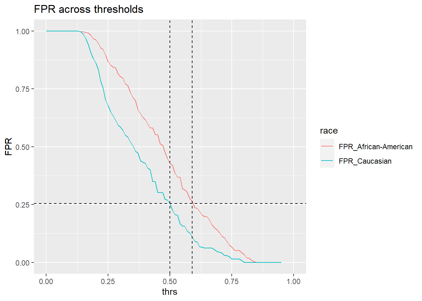
Threshold of 0.59 seems about right. Now that the two groups (Caucasian, African-American) would be at parity we could compute the correct classification rate on the training data data_train.
(Note that we ignored everyone who wasn’t white or black. That’s OK to do, but including other demographics (in any way you like) is OK too).
10.7 Exercise/Homework
- Above we discovered that certain ethnic groups (African-Americans) are treated unfairly by the COMPASS software (as well as or own simply ML model). Please first take the time to read and understand of the lab above.
- Then, please use the code (below) to explore whether we can find similar patterns (unfairness) for other socio-demographic variables, namely
sexandage_catfor the using our prediction model. You can use the models fitted above, i.e., load the data and then run the code in Section 10.1. Subsequently you can use and modify the code below. Below you can find the distribution of in our data. Importantly, identifying whether there is unfairness across gender and age groups is enough for this exercise so the necessary code is in ?@sec-evaluation-our-model but you have to change the grouping variables.
10.8 All the code
# install.packages(pacman)
pacman::p_load(tidyverse,
tidymodels,
knitr,
kableExtra,
DataExplorer,
visdat,
naniar)
load(file = "www/data/data_compas.Rdata")
# install.packages(pacman)
pacman::p_load(tidyverse,
               tidymodels,
               knitr,
               kableExtra,
               DataExplorer,
               visdat,
               naniar)

rm(list=ls())
load(url(sprintf("https://docs.google.com/uc?id=%s&export=download",
                         "1gryEUVDd2qp9Gbgq8G0PDutK_YKKWWIk")))
table(data$race, useNA = "always") %>%
  kable(col.names = c("Race", "Frequency"))
data %>%
  ggplot(aes(x = fct_infreq(race))) + # fct_infreq(): reoder according to frequency
    geom_bar() + # create barplot
    geom_text(stat = "count", # add proportions
            aes(label = round((after_stat(count)) / sum(after_stat(count)), 2),
                vjust = -0.5))
# Extract data with missing outcome
  data_missing_outcome <- data %>% filter(is.na(is_recid_factor))
  dim(data_missing_outcome)
# Omit individuals with missing outcome from data
  data <- data %>% drop_na(is_recid_factor) # ?drop_na
  dim(data)
# Split the data into training and test data
  data_split <- initial_split(data, prop = 0.80)
  data_split # Inspect
# Extract the two datasets
  data_train <- training(data_split)
  data_test <- testing(data_split) # Do not touch until the end!


# Define a recipe for preprocessing (taken from above)
  recipe1 <- recipe(is_recid_factor ~ age + priors_count + race, data = data_train) %>%
    step_normalize(all_numeric_predictors()) %>%
    step_poly(all_numeric_predictors(), degree = 3) # Increase flexibility/parameters

# Define a model
  model1 <- logistic_reg() %>% # logistic model
            set_engine("glm") %>% # define lm package/function
            set_mode("classification")


# Define a workflow
  workflow1 <- workflow() %>% # create empty workflow
    add_recipe(recipe1) %>% # add recipe
    add_model(model1) # add model

# Fit the workflow (including recipe and model)
  fit1 <- workflow1 %>% fit(data = data_train)


# Define metrics
  metrics_combined <- metric_set(accuracy, precision, recall, f_meas,
                                       spec)

# Training data: Add predictions & accuracy
  data_train <- augment(fit1, data_train, type.predict = "response")

  data_train_metrics <- data_train %>%
    select(is_recid_factor, age, .pred_class, .pred_no, .pred_yes) %>%
    metrics_combined(truth = is_recid_factor, estimate = .pred_class)

  # Add FPR
  data_train_metrics <- data_train_metrics %>%
    add_row(.metric = "FPR", .estimator="binary", .estimate = 1-.$.estimate[5])
  # Explain logic -> .$.estimate[5]
  data_train_metrics
# Test data: Add predictions & accuracy
  data_test <- augment(fit1, data_test, type.predict = "response")

  data_test_metrics <- data_test %>%
    select(is_recid_factor, age, .pred_class, .pred_no, .pred_yes) %>%
      metrics_combined(truth = is_recid_factor, estimate = .pred_class)

  # Add FPR
  data_test_metrics <- data_test_metrics %>%
    add_row(.metric = "FPR", .estimator="binary", .estimate = 1-.$.estimate[5])
  data_test_metrics
# Function: False Positive Rate
get_FPR <- function(data_set, # Use assessment or test data here
                    outcome, # Specify outcome variable
                    probability_predicted, # Specify var containting pred. probs.
                    thr) { # Specify threshold
  return( # display results
    # Sum above threshold AND NOT recidivate
    sum((data_set %>% select(dplyr::all_of(probability_predicted)) >= thr) &
      (data_set %>% select(dplyr::all_of(outcome)) == 0), na.rm = TRUE)
    / # divided by
      # Sum NOT recividate
      sum(data_set %>% select(dplyr::all_of(outcome)) == 0, na.rm = TRUE)
  )
}
# Share of people over the threshold that did not recidivate
# of all that did not recidivate (who got falsely predicted to
# recidivate)


# Q: Please explain the function below!

# Function: False Negative Rate
get_FNR <- function(data_set,
                    outcome,
                    probability_predicted,
                    thr) {
  return(
    sum((data_set %>% select(dplyr::all_of(probability_predicted)) < thr) &
      (data_set %>% select(dplyr::all_of(outcome)) == 1), na.rm = TRUE) # ?
    /
      sum(data_set %>% select(dplyr::all_of(outcome)) == 1, na.rm = TRUE)
  ) # ?
}


# Q: Explain the function below!
# Function: Correct Classification Rate
get_CCR <- function(data_set,
                    outcome,
                    probability_predicted,
                    thr) {
  return(
    mean((data_set %>% select(dplyr::all_of(probability_predicted)) >= thr) # ?
    ==
      data_set %>% select(dplyr::all_of(outcome)), na.rm = TRUE)
  ) # ?
}
data_test_all <- data_test %>%
  mutate(race = "All") %>% # replace grouping variable with constant
  nest(.by = "race")
data_test_groups_race <- data_test %>%
  nest(.by = "race")

data_test_groups <- bind_rows(
  data_test_all,
  data_test_groups_race
)
data_test_groups
data_test_groups %>%
  mutate(
    FPR = map_dbl(
      .x = data, # Nested column that includes the datasets
      ~ get_FPR( # Function to get FPR
        data_set = .x,
        outcome = "is_recid",
        probability_predicted = "decile_score",
        thr = 5
      )
    ),
    FNR = map_dbl(
      .x = data,
      ~ get_FNR(
        data_set = .x,
        outcome = "is_recid",
        probability_predicted = "decile_score",
        thr = 5
      )
    ),
    CCR = map_dbl(
      .x = data,
      ~ get_CCR(
        data_set = .x,
        outcome = "is_recid",
        probability_predicted = "decile_score",
        thr = 5
      )
    )
  ) %>%
  mutate_if(is.numeric, round, digits = 2)
data_test_groups <-
  data_test_groups %>%
  mutate(
    FPR = map_dbl(
      .x = data,
      ~ get_FPR(
        data_set = .x,
        outcome = "is_recid",
        probability_predicted = ".pred_yes",
        thr = 0.5
      )
    ),
    FNR = map_dbl(
      .x = data,
      ~ get_FNR(
        data_set = .x,
        outcome = "is_recid",
        probability_predicted = ".pred_yes",
        thr = 0.5
      )
    ),
    CCR = map_dbl(
      .x = data,
      ~ get_CCR(
        data_set = .x,
        outcome = "is_recid",
        probability_predicted = ".pred_yes",
        thr = 0.5
      )
    )
  ) %>%
  mutate_if(is.numeric, round, digits = 2)
# Pivtot the metric results into longformat
data_plot <- data_test_groups %>%
                    select(race, FPR, FNR, CCR) %>%
                    pivot_longer(cols = c("FPR", "FNR", "CCR"),
                                 names_to = "Metric",
                                 values_to = "Estimate")


data_plot %>%
  ggplot(mapping = aes(
    x = Metric,
    y = Estimate,
    color = race
  )) +
  geom_point(size = 3, position=position_dodge(width = .5)) +
  scale_color_brewer(type ="qual") +
  labs(
    title = "Alrgorithmic fairness across ethnic groups",
    x = "Different accuracy metrics",
    y = "Estimate",
    color = "Ethnic groups (race)"
  )
# Define threshold values
thrs <- seq(0, 0.95, 0.01)
thrs
# Expand df with threshold values and calculate rates
data_test_groups %>%
  filter(race != "Native American") %>% # too few observations
  expand(nesting(race, data), thrs) %>%
  mutate(
    FPR = map2_dbl(
      .x = data,
      .y = thrs,
      ~ get_FPR(
        data_set = .x,
        outcome = "is_recid",
        probability_predicted = ".pred_yes",
        thr = .y
      )
    ),
    FNR = map2_dbl(
      .x = data,
      .y = thrs,
      ~ get_FNR(
        data_set = .x,
        outcome = "is_recid",
        probability_predicted = ".pred_yes",
        thr = .y
      )
    ),
    CCR = map2_dbl(
      .x = data,
      .y = thrs,
      ~ get_CCR(
        data_set = .x,
        outcome = "is_recid",
        probability_predicted = ".pred_yes",
        thr = .y
      )
    )
  ) %>%
  pivot_longer(
    cols = FPR:CCR,
    names_to = "measure",
    values_to = "value"
  ) %>%
  ggplot(mapping = aes(
    x = thrs,
    y = value,
    color = measure
  )) +
  geom_smooth(
    se = F,
    method = "loess"
  ) +
  facet_wrap(~race) +
  labs(
    title = "FPR, FNR and CCR across ethnic groups and thresholds",
    x = "(Probability-) Thresholds",
    y = "Measurement values (see legend)",
    color = "Measure"
  )
# Define threshold values
thrs <- seq(0, 0.95, 0.01)

comparison_thresholds <- data_test_groups %>%
  filter(race == "African-American" | race == "Caucasian") %>% # too few observations
  expand(nesting(race, data), thrs) %>%
  mutate(FPR = map2_dbl(
    .x = data,
    .y = thrs,
    ~ get_FPR(
      data_set = .x,
      outcome = "is_recid",
      probability_predicted = ".pred_yes",
      thr = .y
    )
  )) %>%
  select(-data) %>%
  pivot_wider(
    names_from = "race",
    values_from = "FPR",
    names_prefix = "FPR_"
  )

comparison_thresholds %>%
  kable() %>%
  kable_styling("striped", full_width = T) %>%
  scroll_box(height = "200px")
# FPR caucasion at threshold 0.5
threshold_caucasian <- comparison_thresholds$FPR_Caucasian[comparison_thresholds$thrs == 0.5]
round(threshold_caucasian,3)
# Treshold needed for African-Americans to have similar FPR to Caucasians
threshold_African_American <- comparison_thresholds$thrs[which.min(abs(threshold_caucasian - comparison_thresholds$`FPR_African-American`))]
threshold_African_American
comparison_thresholds %>%
  pivot_longer(
    cols = `FPR_African-American`:FPR_Caucasian,
    names_to = "race",
    values_to = "FPR"
  ) %>%
  ggplot() +
  geom_line(
    mapping = aes(
      x = thrs,
      y = FPR,
      color = race
    ),
    method = "loess", se = F
  ) +
  geom_vline(xintercept = 0.5, linetype = "dashed") +
  geom_vline(xintercept = threshold_African_American, linetype = "dashed") +
  geom_hline(yintercept = threshold_caucasian, linetype = "dashed") +
  xlim(0, 1) +
  ylim(0, 1) +
  ggtitle("FPR across thresholds")
data_train.b <- data_train %>% filter(race == "African-American")
data_train.w <- data_train %>% filter(race == "Caucasian")
n.correct <- sum(data_train.b$is_recid == (predict(fit1, new_data = data_train.b, type = "response") > threshold_African_American)) +
sum(data_train.w$is_recid == (predict(fit1, newdata = data_train.w, type = "response") > 0.5))
n.total <- nrow(data_train.b) + nrow(data_train.w)
n.correct / n.total
table(data$sex)
table(data$age_cat)
# Sex
data_test_all <- data_test %>%
mutate(sex = "All") %>% # replace grouping variable with constant
nest(.by = "sex")
data_test_groups_sex <- data_test %>%
nest(.by = "sex")
data_test_groups <- bind_rows(
data_test_all,
data_test_groups_sex
)
data_test_groups %>%
mutate(
FPR = map_dbl(
.x = data,
~ get_FPR(
data_set = .x,
outcome = "is_recid",
probability_predicted = "prediction",
thr = 0.5
)
),
FNR = map_dbl(
.x = data,
~ get_FNR(
data_set = .x,
outcome = "is_recid",
probability_predicted = "prediction",
thr = 0.5
)
),
CCR = map_dbl(
.x = data,
~ get_CCR(
data_set = .x,
outcome = "is_recid",
probability_predicted = "prediction",
thr = 0.5
)
)
) %>%
mutate_if(is.numeric, round, digits = 2)
# age_cat
data_test_all <- data_test %>%
mutate(age_cat = "All") %>% # replace grouping variable with constant
nest(.by = "age_cat")
data_test_groups_age_cat <- data_test %>%
nest(.by = "age_cat")
data_test_groups <- bind_rows(
data_test_all,
data_test_groups_age_cat
)
data_test_groups %>%
mutate(
FPR = map_dbl(
.x = data,
~ get_FPR(
data_set = .x,
outcome = "is_recid",
probability_predicted = "prediction",
thr = 0.5
)
),
FNR = map_dbl(
.x = data,
~ get_FNR(
data_set = .x,
outcome = "is_recid",
probability_predicted = "prediction",
thr = 0.5
)
),
CCR = map_dbl(
.x = data,
~ get_CCR(
data_set = .x,
outcome = "is_recid",
probability_predicted = "prediction",
thr = 0.5
)
)
) %>%
mutate_if(is.numeric, round, digits = 2)
labs = knitr::all_labels()
ignore_chunks <- labs[str_detect(labs, "setup|solution|get-labels|load-local-data")]
labs = setdiff(labs, ignore_chunks)
# Prepare data test keeping relevant variables & predictions
data_test <- data_test %>%
    select(is_recid_factor, age, .pred_class, .pred_no, .pred_yes, race) %>%
  na.omit()

# Create nested dataframe with all observations
data_test_all <- data_test %>%
          mutate(race = "All") %>% # replace grouping variable with constant
          nest(.by = "race")

# Create nested dataframe with grouped observations
data_test_groups <- data_test %>%
          nest(.by = "race")

# Row bind the dataframes
data_test_fairness <- bind_rows(data_test_all,
                                data_test_groups)
data_test_fairness # Inspect nested dataframe
# Calculate metrics for datasets in nested dataframe
data_test_fairness <- data_test_fairness %>%
                      mutate(Metrics = map(
                          .x = data,
                          ~ .x %>%
                            metrics_combined(truth = is_recid_factor,
                                                   estimate = .pred_class) %>%
                            add_row(.metric = "FPR", .estimator="binary", .estimate = 1-.$.estimate[5])))


# Unnest the dataframe

data_test_fairness <- data_test_fairness %>%
                      select(race, Metrics) %>%
                      unnest(Metrics) %>%
                      mutate(.estimate = round(.estimate, 2)) %>%
                      filter(race!="Native American")


# Visualize the results
data_test_fairness %>%
  ggplot(mapping = aes(
    x = .metric,
    y = .estimate,
    color = race
  )) +
  geom_point(size = 3, position=position_dodge(width = .5)) +
  scale_color_brewer(type ="qual") +
  labs(
    title = "Alrgorithmic fairness across ethnic groups",
    x = "Different accuracy metrics",
    y = "Estimate",
    color = "Ethnic groups (race)"
)11 Appendix
11.1 Appendix: Calculating metrics (NEW VERSION)
Let’s now obtain the accuracy (CCR) and the false positive rate (FPR) for our own predictive logistic regression model. Below we focus on the test data data_test. Albeit, if you train a model it could also be interesting to check these metrics during the training process (as not to build an unfair model).
# Prepare data test keeping relevant variables & predictions
data_test <- data_test %>%
select(is_recid_factor, age, .pred_class, .pred_no, .pred_yes, race) %>%
na.omit()
# Create nested dataframe with all observations
data_test_all <- data_test %>%
mutate(race = "All") %>% # replace grouping variable with constant
nest(.by = "race")
# Create nested dataframe with grouped observations
data_test_groups <- data_test %>%
nest(.by = "race")
# Row bind the dataframes
data_test_fairness <- bind_rows(data_test_all,
data_test_groups)
data_test_fairness # Inspect nested dataframe# A tibble: 7 × 2
race data
<chr> <list>
1 All <tibble [1,320 × 5]>
2 African-American <tibble [676 × 5]>
3 Caucasian <tibble [442 × 5]>
4 Hispanic <tibble [128 × 5]>
5 Other <tibble [65 × 5]>
6 Native American <tibble [5 × 5]>
7 Asian <tibble [4 × 5]> # Calculate metrics for datasets in nested dataframe
data_test_fairness <- data_test_fairness %>%
mutate(Metrics = map(
.x = data,
~ .x %>%
metrics_combined(truth = is_recid_factor,
estimate = .pred_class) %>%
add_row(.metric = "FPR", .estimator="binary", .estimate = 1-.$.estimate[5])))
# Unnest the dataframe
data_test_fairness <- data_test_fairness %>%
select(race, Metrics) %>%
unnest(Metrics) %>%
mutate(.estimate = round(.estimate, 2)) %>%
filter(race!="Native American")
# Visualize the results
data_test_fairness %>%
ggplot(mapping = aes(
x = .metric,
y = .estimate,
color = race
)) +
geom_point(size = 3, position=position_dodge(width = .5)) +
scale_color_brewer(type ="qual") +
labs(
title = "Alrgorithmic fairness across ethnic groups",
x = "Different accuracy metrics",
y = "Estimate",
color = "Ethnic groups (race)"
)
References
Footnotes
e.g., forgetting the predictor of ‘prior offenses’↩︎
Simpson’s Paradox can reveal hidden biases within the data that might not be apparent when analyzing the dataset as a whole. When data from different groups are aggregated, it can mask underlying trends that are only visible when the data is segmented. This is particularly important in machine learning, where models trained on aggregated data might inadvertently perpetuate or even amplify these hidden biases, leading to unfair or biased outcomes. Understanding Simpson’s Paradox is crucial for ensuring fairness across different subgroups within the data. Machine learning models need to perform equitably across various demographics, such as gender, race, age, etc.↩︎
A source of statistical bias that can significantly affect the analysis of geographical data. It arises when the results of an analysis change based on the scale or the zoning (i.e., the way in which areas are delineated and aggregated) of the spatial units used in the study.↩︎
e.g., comment length on reddit decreased over time, however, did increase when aggregated according to cohorts↩︎
e.g. only considering links (not content/behavior) in the network could favor low-degree nodes↩︎
is a result of how information is presented↩︎
The idea that top-ranked results are the most relevant and important will result in attraction of more clicks than others. This bias affects search engines/crowdsourcing applications.↩︎
e.g., use of inappropriate and disproportionate benchmarks for evaluation of applications such as Adience and IJB-A benchmarks that were used in the evaluation of facial recognition systems that were biased toward skin color and gender↩︎