Tree-based methods (classification + regression)

Learning outcomes/objective: Learn…

…what decision trees, bagging and random forests are.
…how to use random forests in R.
…how feature selection is automized using those methods.

Source(s): James et al. (2013, chap. 8); Tuning random forest hyperparameters with #TidyTuesday trees data

1 Tree-based methods

See James et al. (2013, chap. 8)
“involve stratifying or segmenting the predictor space into a number of simple regions” (James et al. 2013, 303)
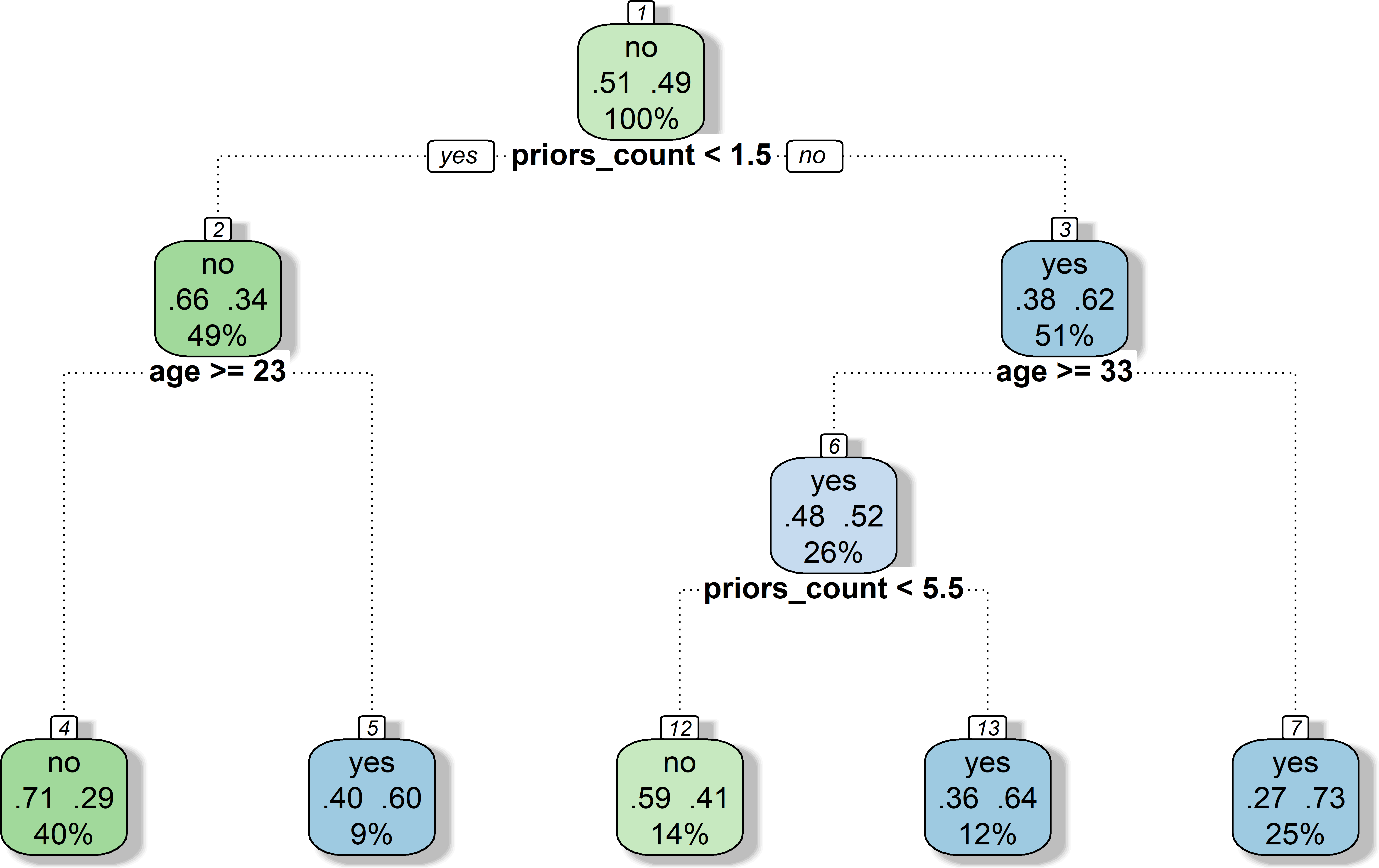
- See Figure 1
  - Region: e.g., 2 variables and 2 cutoffs such as prior offenses (priors_count) (<1.5) followed by age (>=23) → 3 regions/data subsets (Node: 3, 4 and 5)
Prediction for observation $i$
- Based on mean or mode (Q:?) of training observations in the region to which it belongs
Decision tree methods: Name originates from splitting rules that can be summarized in a tree
- Can be applied to both regression and classification problems
- Predictive power of single decision tree not very good
Bagging, random forests,and boosting
- Approaches involve producing multiple trees which are then combined to yield a single consensus prediction (“average prediction”)
- Combination of large number of trees can dramatically increase predictive power, but interpretation is more difficult (black box! Why?!)

Figure 1: Source: Original visualization; For each node: Small white number = number of the node; First line no/yes and color (green, blue) in each node shows majority class; Second line shows proportions of classes, e.g., 0.51 have a no in the first node; Third line shows share of observations in this node, e.g., first node still has 100% of observations in it; yes/no below node indicate whether condition is fullfilled or not;

2 Classification trees

Predict qualitative outcomes rather than a quantitative one (vs. regression trees)
Prediction: Unseen (test) observation $i$ belongs to the most commonly occurring class of training observations (the mode) in the region to which it belongs
- Region: $prior offences < 1.5$ and $age >= 23$
- Training observations: Most individuals in region do NOT re-offended
- Unseen/test observations: Prediction.. also NOT re-offended
To grow classification tree we use recursive splitting/partitioning
- Splitting training data into sub-populations based on several dichotomous independent variables
- Criterion for making binary splits: Classification error rate (vs. RSS in regression tree)
  - minimize CRR: Fraction of training observations in region that do not belong to most common class in region
  - $E=1−\max\limits_{k}(\hat{p}_{mk})$ where $\hat{p}_{mk}$ is proportion of training observations in the $m$th region that are from the $k$th class
  - In practice: Use measures more sensitive to node purity, i.e., Gini index or cross-entropy (cf. James et al. 2013, 312)

3 Regression trees

Regression same logic as classification trees but use RSS as a criterion for making splits (+ min N of observations in final nodes/leaves)
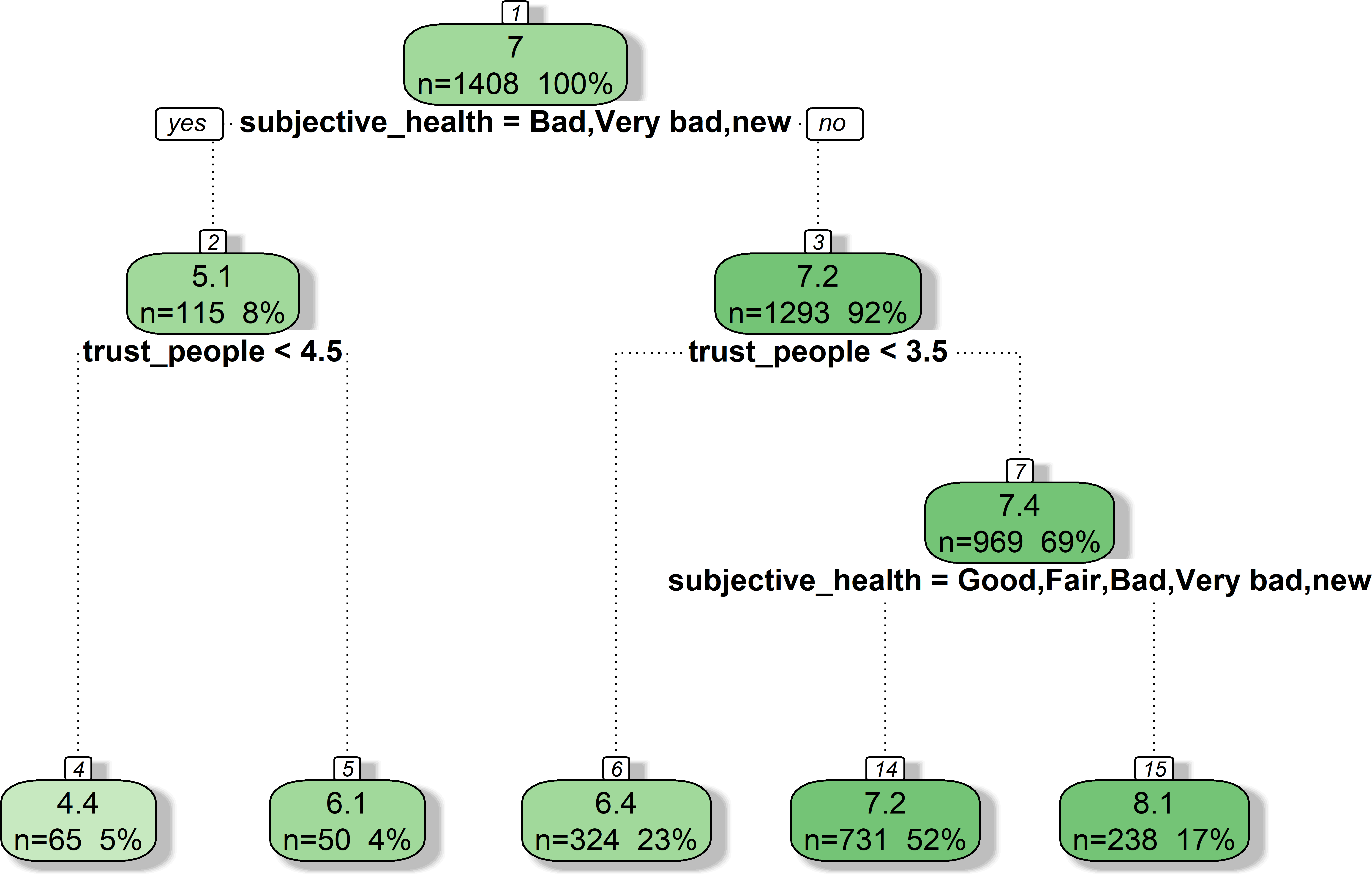
Figure 2 shows an exemplary tree based on our data (ESS: Predicting life_satisfaction)

Figure 2: Source: Original visualization; For each node: Small white number = number of the node; First line = mean of the outcome (life satisfaction 0-10) in this node; Second line shows number of cases in this node both absolut (n) and relative (%), e.g., first node still has 100% of cases namely n=1408; yes/no below node indicate whether condition is fullfilled or not;

4 Advantages and Disadvantages of (single) Trees

Pro (James et al. 2013, Ch. 8.1.4)
- Trees are very easy to explain to people (even easier than linear regression)!
- Decision trees more closely mirror human decision-making than do other regression and classification approaches
- Trees can be displayed graphically, and are easily interpreted even by a non-expert (especially if they are small).
- Trees can easily handle qualitative predictors without the need to create dummy variables.
Contra (James et al. 2013, Ch. 8.1.4)
- Trees generally do not have the same level of predictive accuracy as some other regression and classification approaches
- Trees can be very non-robust: a small change in the data can cause a large change in the final estimated tree.

5 Bagging

Single decision trees may suffer from high variance, i.e., results could be very different for different splits
- Q: Why?
We want: Low variance procedure that yields similar results if applied repeatedly to distinct training datasets (e.g., linear regression)
Bagging: construct $B$ regression trees using $B$ bootstrapped training sets, and average the resulting predictions
- Bootstrap (also called bootstrap aggregation): Take repeated samples from the (single) training set, built predictive model and average predictions
- For Classification Problem: For a given test observation, we can record the class predicted by each of the $B$ trees, and take a majority vote: the overall prediction is the most commonly occurring majority vote class among the $B$ predictions
- For Regression Problem: Average across $B$ predictions

6 Out-of-Bag (OOB) Error Estimation

Out-of-Bag (OBB) Error estimation: Straightforward way to estimate test error of bagged model (no need for cross-validation)
- On average each bagged tree makes use of around two-thirds of the observations
- remaining one-third of observations not used to fit a given bagged tree are referred to as the out-of-bag (OOB) observations
Predict outcome for the $i$th observation using each of the trees in which that observation was OOB
- Will yield around $B/3$ predictions for the $i$th observation
- Then average these predicted responses (if regression is the goal) or take a majority vote (if classification is the goal)
  - Leads to a single OOB prediction for the $i$th observation
  - OOB prediction can be obtained in this way for each of the $n$ observations, from which the overall OOB classification error can be computed (Regression: OOB MSE)
Resulting OOB error is a valid estimate of the test error for the bagged model
- Because outcome/response for each observation is predicted using only the trees that were not fit using that observation
It can be shown that with $B$ sufficiently large, OOB error is virtually equivalent to leave-one-out cross-validation error.
OOB test error approach particularly convenient for large data sets for which cross-validation would be computationally onerous

7 Variable Importance Measures

Variable importance: Which are the most important predictors?
Single decision tree: Intepretation is easy.. just look at the splits in the graph, e.g., Figure 2
Bag of large number of trees: Can’t just visualize single tree and no longer clear which variables are most relevant for splits
- Bagging improves prediction accuracy at the expense of interpretability (James et al. 2013, 319)
Overall summary of importance of each predictor
- Using Gini index (measure of node purity) for bagging classification trees (or RSS for regression trees)
  - Classification trees: Add up the total amount that the Gini index is decreased (i.e., node purity increased) by splits over a given predictor, averaged over all $B$ trees
    - Gini index: a small value indicates that a node contains predominantly observations from a single class
  - See Figure 8.9 (James et al. 2013, 313) for graphical representation of importance: Mean decrease in Gini index for each variable relative to the largest

8 Random forests

Random Forests (RFs) provide improvement over bagged trees
- Decorrelated trees lead to reduction in both test and OOB error over bagging
RFs also build decision trees on bootstrapped training samples but…
….add predictor subsetting:
- Each time a split in a tree is considered,a random sample of $m$ predictors is chosen as split candidates from the full set of $p$ predictors
- Split only allowed to use one of $m$ predictors
- Fresh sample of $m$ predictors taken at each split (typically not all but $m \approx \sqrt{p}$!)
  - On average $(p-m)/p$ splits won’t consider strong predictor (decorrelating trees)
- Objective: Avoid that single strong predictor is always used for first split & decrease correlation of trees
Main difference bagging vs. random forests: Choice of predictor subset size $m$
- RF built using $m=p$ equates Bagging
Recommmendation: Vary $m$ and use small $m$ when predictors are highly correlated
Finally, boosting (skipped here) grows trees sequentially using information from previous trees ee Chapter 8.2.3 (James et al. 2013, 321)

9 Lab: Random forest (regression problem)

Below the steps we would pursue WITHOUT tuning our random forest.
- Step 1: Load data, recode and rename variables
- Step 2: Split the data
- Step 3: Specify recipe, model and workflow
- Step 4: Evaluate model using resampling
- Step 5: Fit final model to full training data and assess accuracy
- Step 6: Fit final model to test data and assess accuracy

9.1 Step 1: Loading, renaming and recoding

See earlier description here (right click and open in new tab).

We first import the data into R:

# install.packages(pacman)
pacman::p_load(tidyverse,
               tidymodels,
               naniar,
               knitr,
               kableExtra,
               DataExplorer,
               visdat)
# Load the .RData file into R
load(url(sprintf("https://docs.google.com/uc?id=%s&export=download",
                         "173VVsu9TZAxsCF_xzBxsxiDQMVc_DdqS")))

9.2 Step 2: Prepare & split the data

Below we split the data and create resampled partitions with vfold_cv() stored in an object called data_folds. Hence, we have the original data_train and data_test but also already resamples of data_train in data_folds.

# Take subset of variables to speed things up!
  data <- data  %>%
    select(life_satisfaction,
           unemployed,
           trust_people,
           education,
           age,
           religion,
           subjective_health) %>%
  mutate(religion = if_else(is.na(religion), "unknown", religion),
         religion = as.factor(religion)) %>%
    drop_na()


# Extract data with missing outcome
  data_missing_outcome <- data %>% filter(is.na(life_satisfaction))
  dim(data_missing_outcome)

[1] 0 7

# Omit individuals with missing outcome from data
  data <- data %>% drop_na(life_satisfaction) # ?drop_na
  dim(data)

[1] 1760    7

# Split the data into training and test data
  set.seed(100)
  data_split <- initial_split(data, prop = 0.80)
  data_split # Inspect

<Training/Testing/Total>
<1408/352/1760>

# Extract the two datasets
  data_train <- training(data_split)
  data_test <- testing(data_split) # Do not touch until the end!

# Create resampled partitions
  set.seed(345)
  data_folds <- vfold_cv(data_train, v = 5) # V-fold/k-fold cross-validation
  data_folds # data_folds now contains several resamples of our training data

#  5-fold cross-validation 
# A tibble: 5 × 2
  splits             id   
  <list>             <chr>
1 <split [1126/282]> Fold1
2 <split [1126/282]> Fold2
3 <split [1126/282]> Fold3
4 <split [1127/281]> Fold4
5 <split [1127/281]> Fold5

Our test data data_test contains 352 observations. The training data (from which we generate the folds) contains 1408 observations.

9.3 Step 3: Specify recipe, model and workflow

Below we define different pre-processing steps in our recipe (see # comments in the chunk):

# Define recipe
recipe1 <- 
  recipe(formula = life_satisfaction ~ ., data = data_train) %>% 
  step_nzv(all_predictors()) %>% # remove variables with zero variances
  step_novel(all_nominal_predictors()) %>% # prepares data to handle previously unseen factor levels 
  #step_dummy(all_nominal_predictors()) %>% # dummy codes categorical variables
  step_zv(all_predictors()) #%>% # remove vars with only single value
  #step_normalize(all_predictors()) # normale predictors

# Inspect the recipe
  recipe1
  
  # Extract and preview data + recipe (direclty with $)
  data_preprocessed <- prep(recipe1, data_train)$template
  dim(data_preprocessed)

[1] 1408    6

Then we specify our random forest model choosing a mode, engine and specifying the workflow with workflow():

# show engines/package that include random forest
show_engines("rand_forest")

# A tibble: 6 × 2
  engine       mode          
  <chr>        <chr>         
1 ranger       classification
2 ranger       regression    
3 randomForest classification
4 randomForest regression    
5 spark        classification
6 spark        regression

# Specify model
model1 <- 
  rand_forest(trees = 1000) %>% # grow 1000 trees!
  set_engine("ranger", 
             importance = "permutation") %>% 
  set_mode("regression")

# Specify workflow
workflow1 <- 
  workflow() %>% 
  add_recipe(recipe1) %>%
  add_model(model1)

9.4 Step 4: Fit/train & evalute model using resampling

Then we fit the random forest to our resamples of the training data (different splits into analysis and assessment data) to be better able to evaluate it accounting for possible variation across subsets:

# Fit the random forest to the cross-validation datasets
fit1 <- workflow1 %>% 
  fit_resamples(resamples = data_folds, # specify cv-datasets
  metrics = metric_set(rmse, rsq, mae)) # save models

And we can evaluate the metrics:

# RMSE and RSQ
collect_metrics(fit1)

# A tibble: 3 × 6
  .metric .estimator  mean     n std_err .config             
  <chr>   <chr>      <dbl> <int>   <dbl> <chr>               
1 mae     standard   1.66      5  0.0475 Preprocessor1_Model1
2 rmse    standard   2.15      5  0.0412 Preprocessor1_Model1
3 rsq     standard   0.104     5  0.0146 Preprocessor1_Model1

Q: What do the different variables and measures stand for?

Insights

.metric = the measures; .estimator = type of estimator; mean = mean of measure across folds; n = number of folds; std_err = standard error across folds; .config = ?
MAE (Mean Absolute Error): This is a measure of the average magnitude of errors between predicted and actual values. It is calculated as the sum of absolute differences between predictions and actuals divided by the total number of data points. MAE is easy to interpret because it represents the average distance between predictions and actuals, but it can be less sensitive to large errors than other measures like RMSE.
RMSE (Root Mean Squared Error): This is another measure of the difference between predicted and actual values that takes into account both the size and direction of the errors. It is calculated as the square root of the mean of squared differences between predictions and actuals. RMSE penalizes larger errors more heavily than smaller ones, making it a useful metric when outliers or extreme values may have a significant impact on model performance. However, its units are not always easily interpreted since they depend on the scale of the dependent variable.
Rsquared ($R^2$): Also known as coefficient of determination, this metric compares the goodness-of-fit of a regression line by measuring the proportion of variance in the dependent variable that can be explained by the independent variables. An $R^2$ score ranges from 0 to 1, with 1 indicating perfect correlation between the predicted and actual values. However, keep in mind that high $R^2$ does not necessarily imply causality or generalizability outside the sample used to train the model.

9.5 Step 5: Fit final model to training data

Once we we are happy with our random forest model (after having used resampling to assess it and potential alternatives) we can fit our workflow that includes the model to the complete training data data_train and also assess it’s accuracy for the training data again.

# Fit final model
fit_final <- fit(workflow1, data = data_train)

# Check accuracy in for full training data
  metrics_combined <- 
    metric_set(rsq, rmse, mae) # Set accuracy metrics


  augment(fit_final, new_data = data_train) %>%
      metrics_combined(truth = life_satisfaction, estimate = .pred)

# A tibble: 3 × 3
  .metric .estimator .estimate
  <chr>   <chr>          <dbl>
1 rsq     standard       0.726
2 rmse    standard       1.35 
3 mae     standard       1.05

Now, we can also explore the variable importance of different predictors and visualize it in Figure 3. The vip() does only like objects of class ranger, hence we have to directly access ist in the layer object using fit_final$fit$fit$fit

# Visualize variable importance
# install.packages("vip")
library(vip)
fit_final$fit$fit$fit %>%
    vip::vip(geom = "point") +
  ylab("Importance of different predictors")+
  xlab("Variables")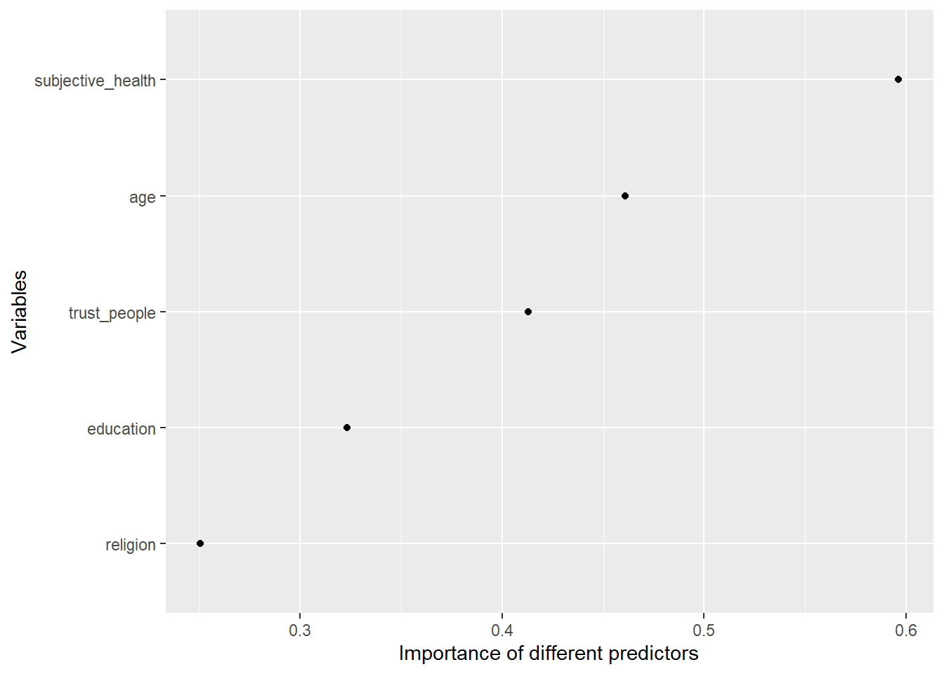

Figure 3: Variable importance for different predictors

Q: What do we see here?

Insights

Figure 3 indicates that trust_people is among the most important predictors.

9.6 Step 6: Fit final model to test data and assess accuracy

We then use the model fit_final fitted/trained on the training data and evaluate the accuracy of this model which is based on the training data using the test data data_test. We use augment() to obtain the predictions:

# Test data: Predictions & accuracy
# Test data: Predictions + accuracy
  regression_metrics <- metric_set(mae, rmse, rsq) # Use several metrics
  
  augment(fit_final , new_data = data_test) %>%
    regression_metrics(truth = life_satisfaction, estimate = .pred)

# A tibble: 3 × 3
  .metric .estimator .estimate
  <chr>   <chr>          <dbl>
1 mae     standard      1.65  
2 rmse    standard      2.21  
3 rsq     standard      0.0405

Q: How does our model compare to the accuracy from the ridge and lasso regression models?

See Regression chapter for suggestions on how to visualize predictions and errors.

10 Exercise: Predicting internet use with a RF

Using the ESS 10 for french citizens, you are interested in building a predictive model of internet_use_time, i.e., the minutes an individual spends on the internet per day. Please use the code above to built a RF model to predict this outcome. Importantly, you are free to use the exact same predictors or add new ones. How well can you predict the outcome?

11 Gradient Boosted Decision Trees (GBDT) & XGBoost

11.1 GBDT & XGBoost vs. Random Forests

Fundamental difference to RFs: Approach to combining decision trees & learning algorithm
Random Forests
- use bootstrap aggregating (or bagging), where decision trees are built independently in parallel
- trees’ predictions are averaged (for regression) or voted (for classification) to produce the final prediction
Gradient Boosted Decision Trees (GBDT)
- use technique called boosting
- trees built sequentially: each new tree aims to correct errors made by previously built trees
  - model learns by fitting new predictor to residual errors made by preceding predictors and not the actual target
  - focuses on reducing both bias and variance by building a series of trees where each tree corrects mistakes of previous one

11.2 Key differences

Model Building:
- RF builds trees independently and combines their predictions, while GBDT builds trees sequentially (each tree learning from mistakes of previous ones)
Objective
- RF aims to reduce variance without increasing bias, while GBDT aims to reduce both bias and variance through iterative corrections
Data Sampling
- In RF each tree is trained on random subset of data; GBDT trains each tree on entire dataset but focuses on instances that were mispredicted by previous trees
Feature Sampling
- RF considers random subset of features for splitting at each node; GBDT typically considers all features when building each tree focusing more on feature importance
Error Correction
- GBDT directly focuses on correcting the errors (minimizing the loss function) from the previous trees, while RF combines diverse trees’ predictions to average out the errors
Random Forest is very robust and often performs well without much hyperparameter tuning. It’s particularly effective for datasets with a lot of noise and is less prone to overfitting.
Gradient Boosted Decision Trees often achieve higher accuracy on complex datasets where performance is critical. However, they are more sensitive to overfitting and require careful tuning of parameters, such as the learning rate and the number of trees.

11.3 GBDT vs. XGBoost (1)

GBDT (Gradient Boosted Decision Trees) and XGBoost (eXtreme Gradient Boosting) are both popular machine learning algorithms
- Both use gradient boosting techniques to build predictive models
- Share same foundational concept of boosting decision trees but have several key differences
Implementation and Efficiency
- GBDT = general term for algorithmic approach of using gradient boosting with decision trees
- XGBoost is a specific, optimized implementation of gradient boosted decision trees designed for speed and performance
  - includes several optimizations in the algorithm and computing for efficiency and scalability
    - e.g., parallelization of tree construction, tree pruning using depth-first approach¹, and handling sparse data
Regularization
- GBDT implementations may not always include options for regularization.
- XGBoost includes built-in L1 (LASSO regression) and L2 (Ridge regression) regularization options

11.4 GBDT vs. XGBoost (2)

Handling Missing Values
- GBDT implementations often require pre-processing of the dataset to handle missing values (imputation or deleting rows/columns)
- XGBoost can handle missing values internally without requiring preprocessing
Flexibility and Scalability
- GBDT generally less flexible in terms of model tuning and scalability
  - Performs well for many tasks but performance and efficiency limited in very large datasets
- XGBoost is highly scalable (single machines AND distributed computing frameworks)
  - Has been engineered to maximize computational efficiency and effectiveness
Hyperparameter Tuning and Model Complexity
- GBDT models can be easier to tune with a fewer number of hyperparameters
- XGBoost provides a wide range of hyperparameters that allow for fine-tuning

12 Lab: XGBoost (regression problem)

# install.packages("xgboost")
library(xgboost)
library(tidyverse)
library(tidymodels)

# Load the .RData file into R
load(url(sprintf("https://docs.google.com/uc?id=%s&export=download",
                         "173VVsu9TZAxsCF_xzBxsxiDQMVc_DdqS")))

# Take subset of variables to speed things up!
  data <- data  %>%
    select(internet_use_time,
           unemployed,
           trust_people,
           education,
           age,
           religion,
           subjective_health) %>%
  mutate(religion = if_else(is.na(religion), "unknown", religion),
         religion = as.factor(religion)) %>%
    drop_na()


# Extract data with missing outcome
  data_missing_outcome <- data %>% filter(is.na(internet_use_time))
  dim(data_missing_outcome)

[1] 0 7

# Omit individuals with missing outcome from data
  data <- data %>% drop_na(internet_use_time) # ?drop_na
  dim(data)

[1] 1591    7

# Split the data into training and test data
  set.seed(100)
  data_split <- initial_split(data, prop = 0.80)
  data_split # Inspect

<Training/Testing/Total>
<1272/319/1591>

# Extract the two datasets
  data_train <- training(data_split)
  data_test <- testing(data_split) # Do not touch until the end!

# Create resampled partitions
  set.seed(345)
  data_folds <- vfold_cv(data_train, v = 5) # V-fold/k-fold cross-validation
  data_folds # data_folds now contains several resamples of our training data

#  5-fold cross-validation 
# A tibble: 5 × 2
  splits             id   
  <list>             <chr>
1 <split [1017/255]> Fold1
2 <split [1017/255]> Fold2
3 <split [1018/254]> Fold3
4 <split [1018/254]> Fold4
5 <split [1018/254]> Fold5

# Define recipe
  recipe1 <- 
    recipe(formula = internet_use_time ~ ., data = data_train) %>% 
    step_nzv(all_predictors()) %>% # remove variables with zero variances
    step_novel(all_nominal_predictors()) %>% # prepares data to handle previously unseen factor levels 
    step_dummy(all_nominal_predictors()) %>% # dummy codes categorical variables
    step_zv(all_predictors()) %>% # remove vars with only single value
    step_normalize(all_predictors()) # normale predictors

# Inspect the recipe
  recipe1
  
  
#  Specify model
set.seed(100)
model1 <- 
  boost_tree(  mode = "regression",
  trees = 200,
  tree_depth = 5,
  learn_rate = 0.05,
  engine = "xgboost") %>% 
  set_mode("regression")

# Specify workflow
workflow1 <- 
  workflow() %>% 
  add_recipe(recipe1) %>%
  add_model(model1)
  

# Fit the random forest to the cross-validation datasets
fit1 <- fit_resamples(
  object = workflow1, # specify workflow
  resamples = data_folds, # specify cv-datasets
  metrics = metric_set(rmse, rsq, mae), # specify metrics to return
  control = control_resamples(verbose = TRUE, # show live comments
                              save_pred = TRUE, # save predictions
                              extract = function(x) extract_fit_engine(x))) # save models


# RMSE and RSQ
collect_metrics(fit1)

# A tibble: 3 × 6
  .metric .estimator    mean     n std_err .config             
  <chr>   <chr>        <dbl> <int>   <dbl> <chr>               
1 mae     standard   128.        5  1.75   Preprocessor1_Model1
2 rmse    standard   173.        5  3.94   Preprocessor1_Model1
3 rsq     standard     0.135     5  0.0137 Preprocessor1_Model1

# Collect average predictions
assessment_data_predictions <- collect_predictions(fit1, summarize = TRUE)
assessment_data_predictions

# A tibble: 1,272 × 4
    .row internet_use_time .config              .pred
   <int>             <dbl> <chr>                <dbl>
 1     1               480 Preprocessor1_Model1 174. 
 2     2               420 Preprocessor1_Model1 259. 
 3     3               120 Preprocessor1_Model1 233. 
 4     4                90 Preprocessor1_Model1 251. 
 5     5                60 Preprocessor1_Model1 319. 
 6     6                90 Preprocessor1_Model1 275. 
 7     7               180 Preprocessor1_Model1 175. 
 8     8                90 Preprocessor1_Model1  70.8
 9     9               480 Preprocessor1_Model1 207. 
10    10               300 Preprocessor1_Model1 226. 
# ℹ 1,262 more rows

# Visualize actual vs. predicted values
assessment_data_predictions %>% 
  ggplot(aes(x = internet_use_time, y = .pred)) + 
  geom_point(alpha = .15) +
  #geom_abline(color = "red") + 
  coord_obs_pred() + 
  ylab("Internet use time (minutes per day): Predicted values") +
  xlab("Internet use time (minutes per day): Actual values") +
  ggtitle("Predictions: Training data")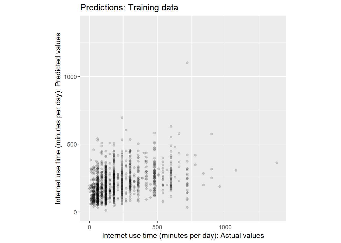

# Fit final model
fit_final <- fit(workflow1, data = data_train)

# Check accuracy in for complete training data
  augment(fit_final, new_data = data_train) %>%
    mae(truth = internet_use_time, estimate = .pred)

# A tibble: 1 × 3
  .metric .estimator .estimate
  <chr>   <chr>          <dbl>
1 mae     standard        91.3

# Visualize variable importance
# install.packages("vip")
library(vip)
fit_final$fit$fit$fit %>%
    vip::vip(geom = "point") +
  ylab("Importance of different predictors")+
  xlab("Variables")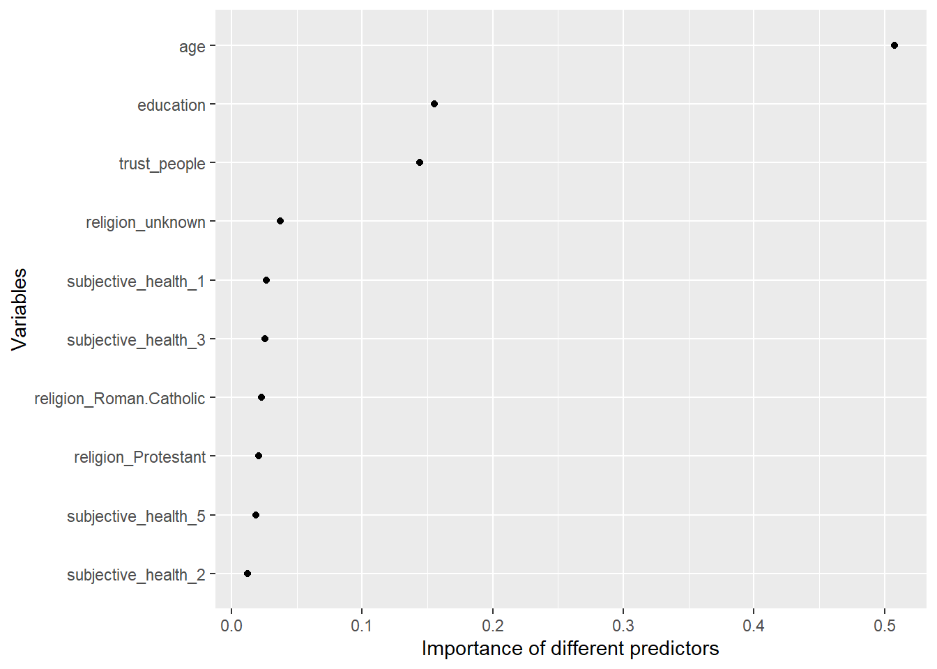

# Test data: Predictions + accuracy
  regression_metrics <- metric_set(mae, rmse, rsq) # Use several metrics
  
  augment(fit_final , new_data = data_test) %>%
    regression_metrics(truth = internet_use_time, estimate = .pred)

# A tibble: 3 × 3
  .metric .estimator .estimate
  <chr>   <chr>          <dbl>
1 mae     standard     123.   
2 rmse    standard     171.   
3 rsq     standard       0.171

13 Exercise: Predicting internet use comparing RF and XGBoost

Above we used both XGBoost to predict internet_use_time. Please set up a script that includes one recipe recipe1, two models (model1 = random forest, model2 = xgboost) and two corresponding workflows (workflow1, workflow2). Train these two workflows and evaluate their accuracy using resampling. Pick the best workflow (and corresponding model), fit it on the whole training data and evaluate the accuracy on the test data.

14 Appendix

14.1 Lab: Random forest (classication problem)

Below you can find and example of building a random forest model for our binary outcome recidivism (without resampling). For more information on the dataset see the corresponding lab on logistic regression for classification).

See earlier description here (right click and open in new tab).

# install.packages(pacman)
pacman::p_load(tidyverse,
               tidymodels,
               knitr,
               kableExtra,
               DataExplorer,
               visdat,
               naniar)

rm(list=ls())
load(url(sprintf("https://docs.google.com/uc?id=%s&export=download",
                         "1gryEUVDd2qp9Gbgq8G0PDutK_YKKWWIk")))

# Extract data with missing outcome
  data_missing_outcome <- data %>% filter(is.na(is_recid_factor))
  dim(data_missing_outcome)

[1] 614  14

# Omit individuals with missing outcome from data
  data <- data %>% drop_na(is_recid_factor) # ?drop_na
  dim(data)

[1] 6600   14

# Split the data into training and test data
  set.seed(100)
  data_split <- initial_split(data, prop = 0.80)
  data_split # Inspect

<Training/Testing/Total>
<5280/1320/6600>

# Extract the two datasets
  data_train <- training(data_split)
  data_test <- testing(data_split) # Do not touch until the end!

# Create resampled partitions
  set.seed(345)
  data_folds <- vfold_cv(data_train, v = 5) # V-fold/k-fold cross-validation
  data_folds # data_folds now contains several resamples of our training data

#  5-fold cross-validation 
# A tibble: 5 × 2
  splits              id   
  <list>              <chr>
1 <split [4224/1056]> Fold1
2 <split [4224/1056]> Fold2
3 <split [4224/1056]> Fold3
4 <split [4224/1056]> Fold4
5 <split [4224/1056]> Fold5

## Step 3: Specify recipe, model and workflow


# Define recipe
recipe1 <- 
  recipe(formula = is_recid_factor ~ age + priors_count + sex + juv_fel_count + juv_misd_count + juv_other_count, data = data_train) %>% 
    step_filter_missing(all_predictors(), threshold = 0.01) %>% 
    step_naomit(is_recid_factor, all_predictors()) %>% # better deal with missings beforehand
    step_nzv(all_predictors(), freq_cut = 0, unique_cut = 0) %>% # remove variables with zero variances
    step_dummy(all_nominal_predictors())

  # Inspect the recipe
    recipe1
  
  # Check preprocessed data
    data_preprocessed <- prep(recipe1, data_train)$template
    dim(data_preprocessed)

[1] 5280    7

# show engines/package that include random forest
show_engines("rand_forest")

# A tibble: 6 × 2
  engine       mode          
  <chr>        <chr>         
1 ranger       classification
2 ranger       regression    
3 randomForest classification
4 randomForest regression    
5 spark        classification
6 spark        regression

# Specify model
model1 <- 
  rand_forest(trees = 1000) %>% # grow 1000 trees!
  set_engine("ranger", 
             importance = "permutation") %>% 
  set_mode("classification")

# Specify workflow
workflow1 <- 
  workflow() %>% 
  add_recipe(recipe1) %>%
  add_model(model1)


## Step 4: Fit/train & evalute model using resampling

# Fit the random forest to the cross-validation datasets
fit1 <- workflow1 %>% 
  fit_resamples(resamples = data_folds, # specify cv-datasets
  metrics = metric_set(accuracy, precision, recall, f_meas)) # save models

# RMSE and RSQ
collect_metrics(fit1)

# A tibble: 4 × 6
  .metric   .estimator  mean     n std_err .config             
  <chr>     <chr>      <dbl> <int>   <dbl> <chr>               
1 accuracy  binary     0.676     5 0.00238 Preprocessor1_Model1
2 f_meas    binary     0.697     5 0.00362 Preprocessor1_Model1
3 precision binary     0.673     5 0.00506 Preprocessor1_Model1
4 recall    binary     0.725     5 0.0111  Preprocessor1_Model1

## Step 5: Fit final model to training data


# Fit final model
fit_final <- fit(workflow1, data = data_train)

# Check accuracy in for full training data
  metrics_combined <- 
    metric_set(accuracy, precision, recall, f_meas) # Set accuracy metrics

  data_train %>%
    augment(x = fit_final, type.predict = "response") %>%
        metrics_combined(truth = is_recid_factor, estimate = .pred_class)

# A tibble: 4 × 3
  .metric   .estimator .estimate
  <chr>     <chr>          <dbl>
1 accuracy  binary         0.708
2 precision binary         0.701
3 recall    binary         0.754
4 f_meas    binary         0.727

# Confusion matrix
  data_train %>%
    augment(x = fit_final, type.predict = "response") %>%
        conf_mat(truth = is_recid_factor, estimate = .pred_class)

          Truth
Prediction   no  yes
       no  2049  872
       yes  670 1689

# Visualize variable importance
# install.packages("vip")
library(vip)
fit_final$fit$fit$fit %>%
    vip::vip(geom = "point") +
  ylab("Importance of different predictors")+
  xlab("Variables")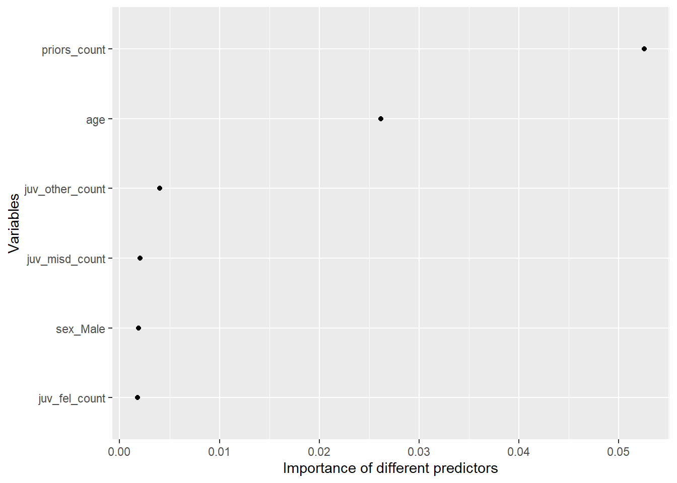

# Test data: Predictions + accuracy
  data_test %>%
    augment(x = fit_final, type.predict = "response") %>%
        metrics_combined(truth = is_recid_factor, estimate = .pred_class)

# A tibble: 4 × 3
  .metric   .estimator .estimate
  <chr>     <chr>          <dbl>
1 accuracy  binary         0.686
2 precision binary         0.701
3 recall    binary         0.714
4 f_meas    binary         0.708

15 All the code

# install.packages(pacman)
pacman::p_load(tidyverse,
               tidymodels,
               naniar,
               knitr,
               kableExtra,
               DataExplorer,
               visdat)
load(file = "www/data/data_ess.Rdata")
# install.packages(pacman)
pacman::p_load(tidyverse,
               tidymodels,
               naniar,
               knitr,
               kableExtra,
               DataExplorer,
               visdat)
# Load the .RData file into R
load(url(sprintf("https://docs.google.com/uc?id=%s&export=download",
                         "173VVsu9TZAxsCF_xzBxsxiDQMVc_DdqS")))
# Take subset of variables to speed things up!
  data <- data  %>%
    select(life_satisfaction,
           unemployed,
           trust_people,
           education,
           age,
           religion,
           subjective_health) %>%
  mutate(religion = if_else(is.na(religion), "unknown", religion),
         religion = as.factor(religion)) %>%
    drop_na()


# Extract data with missing outcome
  data_missing_outcome <- data %>% filter(is.na(life_satisfaction))
  dim(data_missing_outcome)

# Omit individuals with missing outcome from data
  data <- data %>% drop_na(life_satisfaction) # ?drop_na
  dim(data)

# Split the data into training and test data
  set.seed(100)
  data_split <- initial_split(data, prop = 0.80)
  data_split # Inspect

# Extract the two datasets
  data_train <- training(data_split)
  data_test <- testing(data_split) # Do not touch until the end!

# Create resampled partitions
  set.seed(345)
  data_folds <- vfold_cv(data_train, v = 5) # V-fold/k-fold cross-validation
  data_folds # data_folds now contains several resamples of our training data  
# Define recipe
recipe1 <- 
  recipe(formula = life_satisfaction ~ ., data = data_train) %>% 
  step_nzv(all_predictors()) %>% # remove variables with zero variances
  step_novel(all_nominal_predictors()) %>% # prepares data to handle previously unseen factor levels 
  #step_dummy(all_nominal_predictors()) %>% # dummy codes categorical variables
  step_zv(all_predictors()) #%>% # remove vars with only single value
  #step_normalize(all_predictors()) # normale predictors

# Inspect the recipe
  recipe1
  
  # Extract and preview data + recipe (direclty with $)
  data_preprocessed <- prep(recipe1, data_train)$template
  dim(data_preprocessed)
# show engines/package that include random forest
show_engines("rand_forest")

# Specify model
model1 <- 
  rand_forest(trees = 1000) %>% # grow 1000 trees!
  set_engine("ranger", 
             importance = "permutation") %>% 
  set_mode("regression")

# Specify workflow
workflow1 <- 
  workflow() %>% 
  add_recipe(recipe1) %>%
  add_model(model1)
# Fit the random forest to the cross-validation datasets
fit1 <- workflow1 %>% 
  fit_resamples(resamples = data_folds, # specify cv-datasets
  metrics = metric_set(rmse, rsq, mae)) # save models
# library(rpart)
# library(rpart.plot)
library(rattle)
library(magick)

tree <- decision_tree() %>%
   set_engine("rpart") %>%
   set_mode("regression")

 tree_wf <- workflow() %>%
   add_recipe(recipe1) %>%
   add_model(tree) %>%
   fit(data_train) #results are found here

 tree_fit <- tree_wf %>%
  pull_workflow_fit()
 
 #rpart.plot(tree_fit$fit)
 
 png(file = "regression_tree_example.png",   
  width     = 7,
  height    = 6,
  units     = "in",
    res = 1000)
 
 
 fancyRpartPlot(tree_fit$fit,cex=0.8, main = "", caption = "")
 dev.off()
 
 
 img <- image_read("regression_tree_example.png")
 img <- image_trim(img)
 image_write(image = img,
             path = "regression_tree_example.png",format="png")
 
# RMSE and RSQ
collect_metrics(fit1)
# Fit final model
fit_final <- fit(workflow1, data = data_train)

# Check accuracy in for full training data
  metrics_combined <- 
    metric_set(rsq, rmse, mae) # Set accuracy metrics


  augment(fit_final, new_data = data_train) %>%
      metrics_combined(truth = life_satisfaction, estimate = .pred)  
  
# Visualize variable importance
# install.packages("vip")
library(vip)
fit_final$fit$fit$fit %>%
    vip::vip(geom = "point") +
  ylab("Importance of different predictors")+
  xlab("Variables")
# Test data: Predictions & accuracy
# Test data: Predictions + accuracy
  regression_metrics <- metric_set(mae, rmse, rsq) # Use several metrics
  
  augment(fit_final , new_data = data_test) %>%
    regression_metrics(truth = life_satisfaction, estimate = .pred)
# install.packages("xgboost")
library(xgboost)
library(tidyverse)
library(tidymodels)

# Load the .RData file into R
load(url(sprintf("https://docs.google.com/uc?id=%s&export=download",
                         "173VVsu9TZAxsCF_xzBxsxiDQMVc_DdqS")))

# Take subset of variables to speed things up!
  data <- data  %>%
    select(internet_use_time,
           unemployed,
           trust_people,
           education,
           age,
           religion,
           subjective_health) %>%
  mutate(religion = if_else(is.na(religion), "unknown", religion),
         religion = as.factor(religion)) %>%
    drop_na()


# Extract data with missing outcome
  data_missing_outcome <- data %>% filter(is.na(internet_use_time))
  dim(data_missing_outcome)

# Omit individuals with missing outcome from data
  data <- data %>% drop_na(internet_use_time) # ?drop_na
  dim(data)

# Split the data into training and test data
  set.seed(100)
  data_split <- initial_split(data, prop = 0.80)
  data_split # Inspect

# Extract the two datasets
  data_train <- training(data_split)
  data_test <- testing(data_split) # Do not touch until the end!

# Create resampled partitions
  set.seed(345)
  data_folds <- vfold_cv(data_train, v = 5) # V-fold/k-fold cross-validation
  data_folds # data_folds now contains several resamples of our training data  
  
  
  
  
# Define recipe
  recipe1 <- 
    recipe(formula = internet_use_time ~ ., data = data_train) %>% 
    step_nzv(all_predictors()) %>% # remove variables with zero variances
    step_novel(all_nominal_predictors()) %>% # prepares data to handle previously unseen factor levels 
    step_dummy(all_nominal_predictors()) %>% # dummy codes categorical variables
    step_zv(all_predictors()) %>% # remove vars with only single value
    step_normalize(all_predictors()) # normale predictors

# Inspect the recipe
  recipe1
  
  
#  Specify model
set.seed(100)
model1 <- 
  boost_tree(  mode = "regression",
  trees = 200,
  tree_depth = 5,
  learn_rate = 0.05,
  engine = "xgboost") %>% 
  set_mode("regression")

# Specify workflow
workflow1 <- 
  workflow() %>% 
  add_recipe(recipe1) %>%
  add_model(model1)
  

# Fit the random forest to the cross-validation datasets
fit1 <- fit_resamples(
  object = workflow1, # specify workflow
  resamples = data_folds, # specify cv-datasets
  metrics = metric_set(rmse, rsq, mae), # specify metrics to return
  control = control_resamples(verbose = TRUE, # show live comments
                              save_pred = TRUE, # save predictions
                              extract = function(x) extract_fit_engine(x))) # save models


# RMSE and RSQ
collect_metrics(fit1)

# Collect average predictions
assessment_data_predictions <- collect_predictions(fit1, summarize = TRUE)
assessment_data_predictions


# Visualize actual vs. predicted values
assessment_data_predictions %>% 
  ggplot(aes(x = internet_use_time, y = .pred)) + 
  geom_point(alpha = .15) +
  #geom_abline(color = "red") + 
  coord_obs_pred() + 
  ylab("Internet use time (minutes per day): Predicted values") +
  xlab("Internet use time (minutes per day): Actual values") +
  ggtitle("Predictions: Training data")



# Fit final model
fit_final <- fit(workflow1, data = data_train)

# Check accuracy in for complete training data
  augment(fit_final, new_data = data_train) %>%
    mae(truth = internet_use_time, estimate = .pred)
  
  
# Visualize variable importance
# install.packages("vip")
library(vip)
fit_final$fit$fit$fit %>%
    vip::vip(geom = "point") +
  ylab("Importance of different predictors")+
  xlab("Variables")



# Test data: Predictions + accuracy
  regression_metrics <- metric_set(mae, rmse, rsq) # Use several metrics
  
  augment(fit_final , new_data = data_test) %>%
    regression_metrics(truth = internet_use_time, estimate = .pred)
# install.packages(pacman)
pacman::p_load(tidyverse,
               tidymodels,
               knitr,
               kableExtra,
               DataExplorer,
               visdat,
               naniar)
load(file = "www/data/data_compas.Rdata")
# install.packages(pacman)
pacman::p_load(tidyverse,
               tidymodels,
               knitr,
               kableExtra,
               DataExplorer,
               visdat,
               naniar)

rm(list=ls())
load(url(sprintf("https://docs.google.com/uc?id=%s&export=download",
                         "1gryEUVDd2qp9Gbgq8G0PDutK_YKKWWIk")))
# Extract data with missing outcome
  data_missing_outcome <- data %>% filter(is.na(is_recid_factor))
  dim(data_missing_outcome)

# Omit individuals with missing outcome from data
  data <- data %>% drop_na(is_recid_factor) # ?drop_na
  dim(data)

# Split the data into training and test data
  set.seed(100)
  data_split <- initial_split(data, prop = 0.80)
  data_split # Inspect

# Extract the two datasets
  data_train <- training(data_split)
  data_test <- testing(data_split) # Do not touch until the end!

# Create resampled partitions
  set.seed(345)
  data_folds <- vfold_cv(data_train, v = 5) # V-fold/k-fold cross-validation
  data_folds # data_folds now contains several resamples of our training data  


## Step 3: Specify recipe, model and workflow


# Define recipe
recipe1 <- 
  recipe(formula = is_recid_factor ~ age + priors_count + sex + juv_fel_count + juv_misd_count + juv_other_count, data = data_train) %>% 
    step_filter_missing(all_predictors(), threshold = 0.01) %>% 
    step_naomit(is_recid_factor, all_predictors()) %>% # better deal with missings beforehand
    step_nzv(all_predictors(), freq_cut = 0, unique_cut = 0) %>% # remove variables with zero variances
    step_dummy(all_nominal_predictors())

  # Inspect the recipe
    recipe1
  
  # Check preprocessed data
    data_preprocessed <- prep(recipe1, data_train)$template
    dim(data_preprocessed)

# show engines/package that include random forest
show_engines("rand_forest")

# Specify model
model1 <- 
  rand_forest(trees = 1000) %>% # grow 1000 trees!
  set_engine("ranger", 
             importance = "permutation") %>% 
  set_mode("classification")

# Specify workflow
workflow1 <- 
  workflow() %>% 
  add_recipe(recipe1) %>%
  add_model(model1)


## Step 4: Fit/train & evalute model using resampling

# Fit the random forest to the cross-validation datasets
fit1 <- workflow1 %>% 
  fit_resamples(resamples = data_folds, # specify cv-datasets
  metrics = metric_set(accuracy, precision, recall, f_meas)) # save models

# RMSE and RSQ
collect_metrics(fit1)

## Step 5: Fit final model to training data


# Fit final model
fit_final <- fit(workflow1, data = data_train)

# Check accuracy in for full training data
  metrics_combined <- 
    metric_set(accuracy, precision, recall, f_meas) # Set accuracy metrics

  data_train %>%
    augment(x = fit_final, type.predict = "response") %>%
        metrics_combined(truth = is_recid_factor, estimate = .pred_class)


# Confusion matrix
  data_train %>%
    augment(x = fit_final, type.predict = "response") %>%
        conf_mat(truth = is_recid_factor, estimate = .pred_class)
  

# Visualize variable importance
# install.packages("vip")
library(vip)
fit_final$fit$fit$fit %>%
    vip::vip(geom = "point") +
  ylab("Importance of different predictors")+
  xlab("Variables")



# Test data: Predictions + accuracy
  data_test %>%
    augment(x = fit_final, type.predict = "response") %>%
        metrics_combined(truth = is_recid_factor, estimate = .pred_class)
# library(rpart)
# library(rpart.plot)
library(rattle)
library(magick)

tree <- decision_tree() %>%
   set_engine("rpart") %>%
   set_mode("classification")

 tree_wf <- workflow() %>%
   add_recipe(recipe1) %>%
   add_model(tree) %>%
   fit(data_train) #results are found here

 tree_fit <- tree_wf %>%
  pull_workflow_fit()
 
 #rpart.plot(tree_fit$fit)
 
 png(file = "classification_tree_example.png",   
  width     = 7,
  height    = 6,
  units     = "in",
    res = 1000)
 
 
 fancyRpartPlot(tree_fit$fit,cex=0.8, main = "", caption = "")
 dev.off()
 
 
 img <- image_read("classification_tree_example.png")
 img <- image_trim(img)
 image_write(image = img,
             path = "classification_tree_example.png",format="png")

labs = knitr::all_labels()
ignore_chunks <- labs[str_detect(labs, "exclude|setup|solution|get-labels")]
labs = setdiff(labs, ignore_chunks)

References

James, Gareth, Daniela Witten, Trevor Hastie, and Robert Tibshirani. 2013. An Introduction to Statistical Learning: With Applications in R. Springer Texts in Statistics. Springer.

Footnotes

XGBoost employs a depth-first approach for tree pruning, where it grows the tree vertically by exploring as far down a given branch as possible before backtracking to explore another branch. This technique helps in managing the complexity of the model by removing splits that contribute less to the prediction accuracy, thus optimizing the model’s performance and preventing overfitting.↩︎