Data exploration
Learning outcomes/objective: Learn…
- …why data exploration is a necessary step in building predictive models.
- …how to explore a dataset in R visually and with descriptive statistics.
- …get to know the datasets we use in this workshop (ESS data, COMPAS data).
- …a few cool new packages/functions in R.
1 Why Data Exploration?
- Fundamental step before modeling
- Ensures understanding of dataset characteristics
- Identifies anomalies and outliers that could affect model performance
2 Objectives of Data Exploration
- Understanding the dataset
- Types of variables (numerical, categorical)
- Distribution of variables
- Identifying Issues
- Missing values
- Outliers and anomalies
- Potential biases & non-representativness (e.g., only males included)
- Preparation oneself for modeling (later)
- Feature selection (e.g., drop vars with many missings)
- Data transformation and normalization
- Choosing the right model based on data characteristics
3 Data Exploration Techniques
- Statistical summaries
- Descriptive statistics (mean, median, mode, standard deviation)
- Correlation analysis
- Visualization tools
- Histograms/barplots for distribution
- Box plots for outliers
- Scatter plots for relationships
- Handling missing data
- Techniques: imputation, deletion, and understanding the impact on the model
4 Lab: Exploring a dataset (ESS data)
4.1 The data (ESS)
We use the European Social Survey (ESS) [Round 10 - 2020. Democracy, Digital social contacts] to tackle ML regression problems with a continuous outcome. The ESS (prepared by myself1) contains different outcomes amenable to both classification and regression as well as a lot of variables that could be used as features (~380 variables). We are interested in predicting the outcome life_satisfaction using different potential predictors.
life_satisfaction = stflife: measures life satisfaction (How satisfied with life as a whole?).unemployed = uempla: measures unemployment (Doing last 7 days: unemployed, actively looking for job).education = eisced: measures education (Highest level of education, ES - ISCED).age: measures age etc.country = cntry: measures a respondent’s country of origin (here held constant for France).- etc.
We first import the data into R:
4.2 Exploring using descriptive statistics
Here we use function from the skimr and the modelsummary package.
Q: Please quickly go through the statistics below. How can we interpret them? What do they tell us about the data? Can you spot anything interesting?
library(skimr)
library(modelsummary)
# Data overview
# skim(data) # Run this in R (output is too long)
datasummary_skim(data, type = "numeric")| Unique (#) | Missing (%) | Mean | SD | Min | Median | Max | ||
|---|---|---|---|---|---|---|---|---|
| respondent_id | 1977 | 0 | 18947.9 | 5193.1 | 10005.0 | 18927.0 | 27908.0 |  |
| life_satisfaction | 12 | 10 | 7.0 | 2.2 | 0.0 | 8.0 | 10.0 |  |
| unemployed_active | 2 | 0 | 0.0 | 0.2 | 0.0 | 0.0 | 1.0 |  |
| unemployed | 2 | 0 | 0.0 | 0.1 | 0.0 | 0.0 | 1.0 |  |
| education | 8 | 1 | 3.1 | 1.9 | 0.0 | 3.0 | 6.0 |  |
| news_politics_minutes | 88 | 0 | 84.3 | 144.1 | 0.0 | 60.0 | 1200.0 |  |
| internet_use_time | 59 | 19 | 209.6 | 183.0 | 0.0 | 150.0 | 1380.0 |  |
| trust_people | 12 | 0 | 4.7 | 2.1 | 0.0 | 5.0 | 10.0 |  |
| people_fair | 12 | 0 | 6.0 | 2.0 | 0.0 | 6.0 | 10.0 |  |
| people_helpful | 12 | 0 | 4.8 | 2.1 | 0.0 | 5.0 | 10.0 |  |
| trust_parliament | 12 | 3 | 4.5 | 2.4 | 0.0 | 5.0 | 10.0 |  |
| trust_legal_system | 12 | 1 | 5.2 | 2.5 | 0.0 | 5.0 | 10.0 |  |
| trust_police | 12 | 0 | 6.4 | 2.2 | 0.0 | 7.0 | 10.0 |  |
| trust_politicians | 12 | 1 | 3.9 | 2.2 | 0.0 | 4.0 | 10.0 |  |
| trust_political_parties | 12 | 2 | 3.4 | 2.1 | 0.0 | 3.0 | 10.0 |  |
| trust_european_parliament | 12 | 6 | 4.4 | 2.4 | 0.0 | 5.0 | 10.0 |  |
| trust_united_nations | 12 | 7 | 5.2 | 2.4 | 0.0 | 5.0 | 10.0 |  |
| voted_national_election | 3 | 18 | 0.4 | 0.5 | 0.0 | 0.0 | 1.0 |  |
| contacted_politician | 3 | 0 | 0.9 | 0.3 | 0.0 | 1.0 | 1.0 |  |
| donated_political_party | 3 | 0 | 1.0 | 0.2 | 0.0 | 1.0 | 1.0 |  |
| campaign_badge | 3 | 0 | 0.9 | 0.3 | 0.0 | 1.0 | 1.0 |  |
| signed_petition | 3 | 0 | 0.7 | 0.4 | 0.0 | 1.0 | 1.0 |  |
| public_demonstration | 3 | 0 | 0.9 | 0.3 | 0.0 | 1.0 | 1.0 |  |
| boycotted_products | 3 | 1 | 0.7 | 0.5 | 0.0 | 1.0 | 1.0 |  |
| posted_politics_online | 3 | 0 | 0.8 | 0.4 | 0.0 | 1.0 | 1.0 |  |
| volunteered_charity | 2 | 0 | 0.7 | 0.4 | 0.0 | 1.0 | 1.0 |  |
| feel_close_party | 3 | 2 | 0.6 | 0.5 | 0.0 | 1.0 | 1.0 |  |
| left_right_scale | 12 | 11 | 5.1 | 2.2 | 0.0 | 5.0 | 10.0 |  |
| satisfied_economy | 12 | 3 | 4.6 | 2.2 | 0.0 | 5.0 | 10.0 |  |
| satisfied_government | 12 | 3 | 4.8 | 2.3 | 0.0 | 5.0 | 10.0 |  |
| satisfied_democracy | 12 | 2 | 5.2 | 2.4 | 0.0 | 5.0 | 10.0 |  |
| state_education | 12 | 3 | 5.1 | 2.2 | 0.0 | 5.0 | 10.0 |  |
| state_health_services | 12 | 0 | 6.3 | 2.3 | 0.0 | 7.0 | 10.0 |  |
| eu_unification | 12 | 7 | 5.5 | 2.6 | 0.0 | 5.0 | 10.0 |  |
| immigration_economy | 12 | 3 | 5.4 | 2.4 | 0.0 | 5.0 | 10.0 |  |
| immigration_cultural_life | 12 | 2 | 5.8 | 2.7 | 0.0 | 6.0 | 10.0 |  |
| immigrants_country_impact | 12 | 2 | 5.2 | 2.2 | 0.0 | 5.0 | 10.0 |  |
| happiness | 12 | 0 | 7.4 | 1.7 | 0.0 | 8.0 | 10.0 |  |
| crime_victim_last_5_years | 3 | 0 | 0.8 | 0.4 | 0.0 | 1.0 | 1.0 |  |
| attachment_country | 12 | 0 | 8.0 | 1.9 | 0.0 | 8.0 | 10.0 |  |
| attachment_europe | 12 | 1 | 6.1 | 2.5 | 0.0 | 6.0 | 10.0 |  |
| religion_current | 3 | 1 | 0.5 | 0.5 | 0.0 | 0.0 | 1.0 |  |
| ever_religion | 3 | 51 | 0.8 | 0.4 | 0.0 | 1.0 | 1.0 |  |
| religiousness | 12 | 1 | 4.7 | 3.5 | 0.0 | 5.0 | 10.0 |  |
| discrimination_group_membership | 3 | 1 | 0.9 | 0.3 | 0.0 | 1.0 | 1.0 |  |
| discrimination_colour_race | 2 | 0 | 0.0 | 0.2 | 0.0 | 0.0 | 1.0 |  |
| discrimination_nationality | 2 | 0 | 0.0 | 0.1 | 0.0 | 0.0 | 1.0 |  |
| discrimination_religion | 2 | 0 | 0.0 | 0.2 | 0.0 | 0.0 | 1.0 |  |
| discrimination_language | 2 | 0 | 0.0 | 0.1 | 0.0 | 0.0 | 1.0 |  |
| discrimination_ethnic_group | 2 | 0 | 0.0 | 0.1 | 0.0 | 0.0 | 1.0 |  |
| discrimination_age | 2 | 0 | 0.0 | 0.1 | 0.0 | 0.0 | 1.0 |  |
| discrimination_gender | 2 | 0 | 0.0 | 0.2 | 0.0 | 0.0 | 1.0 |  |
| discrimination_sexuality | 2 | 0 | 0.0 | 0.1 | 0.0 | 0.0 | 1.0 |  |
| discrimination_disability | 2 | 0 | 0.0 | 0.1 | 0.0 | 0.0 | 1.0 |  |
| discrimination_other | 2 | 0 | 0.0 | 0.2 | 0.0 | 0.0 | 1.0 | |
| discrimination_not_applicable | 2 | 0 | 0.9 | 0.3 | 0.0 | 1.0 | 1.0 |  |
| citizenship_country | 3 | 0 | 0.1 | 0.2 | 0.0 | 0.0 | 1.0 |  |
| born_in_country | 2 | 0 | 0.1 | 0.3 | 0.0 | 0.0 | 1.0 |  |
| year_first_live_in_country | 74 | 88 | 1991.1 | 19.9 | 1937.0 | 1995.0 | 2019.0 |  |
| feel_ethnic_group_part | 3 | 3 | 0.1 | 0.4 | 0.0 | 0.0 | 1.0 |  |
| father_born_in_country | 3 | 1 | 0.2 | 0.4 | 0.0 | 0.0 | 1.0 |  |
| mother_born_in_country | 3 | 0 | 0.2 | 0.4 | 0.0 | 0.0 | 1.0 |  |
| climate_change_personal_responsibility | 12 | 1 | 7.5 | 2.1 | 0.0 | 8.0 | 10.0 |  |
| energy_use_impact_climate_change | 12 | 66 | 6.2 | 2.2 | 0.0 | 6.0 | 10.0 |  |
| people_limit_energy_use_likelihood | 12 | 66 | 4.2 | 1.9 | 0.0 | 4.0 | 10.0 |  |
| government_action_reduce_climate_change | 12 | 66 | 4.4 | 2.1 | 0.0 | 5.0 | 10.0 |  |
| elections_free_fair | 12 | 2 | 8.7 | 1.7 | 0.0 | 9.0 | 10.0 |  |
| political_parties_clear_alternatives | 12 | 2 | 8.4 | 1.8 | 0.0 | 9.0 | 10.0 |  |
| media_free_criticism_government | 12 | 1 | 7.9 | 2.3 | 0.0 | 8.0 | 10.0 |  |
| minority_rights_protection | 12 | 2 | 8.4 | 1.8 | 0.0 | 9.0 | 10.0 |  |
| citizen_final_say_referendums | 12 | 3 | 7.6 | 2.1 | 0.0 | 8.0 | 10.0 |  |
| courts_equal_treatment | 12 | 1 | 9.1 | 1.4 | 0.0 | 10.0 | 10.0 |  |
| governing_parties_punished_bad_job | 12 | 2 | 8.5 | 1.9 | 0.0 | 9.0 | 10.0 |  |
| government_protection_against_poverty | 12 | 1 | 8.7 | 1.7 | 0.0 | 9.0 | 10.0 |  |
| government_income_level_measures | 12 | 2 | 8.0 | 2.1 | 0.0 | 8.0 | 10.0 |  |
| ordinary_people_views_prevail | 12 | 4 | 7.4 | 2.0 | 0.0 | 8.0 | 10.0 |  |
| people_will_cannot_be_stopped | 12 | 2 | 7.4 | 2.2 | 0.0 | 8.0 | 10.0 |  |
| key_decisions_by_national_government | 12 | 4 | 7.4 | 2.0 | 0.0 | 8.0 | 10.0 |  |
| free_fair_elections | 12 | 4 | 7.2 | 2.3 | 0.0 | 8.0 | 10.0 |  |
| clear_political_alternatives | 12 | 3 | 5.1 | 2.2 | 0.0 | 5.0 | 10.0 |  |
| media_freedom_criticism | 12 | 2 | 6.4 | 2.6 | 0.0 | 7.0 | 10.0 |  |
| minority_rights_protection_incountry | 12 | 4 | 5.9 | 2.2 | 0.0 | 6.0 | 10.0 |  |
| direct_voting_referendums | 12 | 4 | 3.8 | 2.6 | 0.0 | 4.0 | 10.0 |  |
| courts_equality | 12 | 3 | 4.4 | 2.6 | 0.0 | 4.0 | 10.0 |  |
| governing_party_punishment | 12 | 6 | 5.0 | 2.7 | 0.0 | 5.0 | 10.0 |  |
| government_protection_poverty | 12 | 2 | 4.4 | 2.4 | 0.0 | 4.0 | 10.0 |  |
| income_inequality_reduction | 12 | 4 | 4.3 | 2.2 | 0.0 | 4.0 | 10.0 |  |
| ordinary_people_influence | 12 | 5 | 3.6 | 2.2 | 0.0 | 4.0 | 10.0 |  |
| unstoppable_public_will | 12 | 3 | 3.6 | 2.4 | 0.0 | 4.0 | 10.0 |  |
| national_vs_eu_decisions | 12 | 8 | 5.5 | 2.2 | 0.0 | 6.0 | 10.0 |  |
| democracy_importance_policy_change | 11 | 37 | 7.5 | 1.6 | 0.0 | 8.0 | 10.0 |  |
| democracy_government_policy_change_country | 12 | 23 | 4.4 | 2.3 | 0.0 | 5.0 | 10.0 |  |
| democracy_importance_stick_to_policies | 12 | 80 | 7.0 | 1.7 | 0.0 | 7.0 | 10.0 |  |
| democracy_stick_to_policies_country | 12 | 80 | 6.5 | 1.8 | 0.0 | 7.0 | 10.0 |  |
| showcard_correct_version | 1 | 0 | 1.0 | 0.0 | 1.0 | 1.0 | 1.0 |  |
| importance_live_democracy | 12 | 2 | 8.5 | 2.0 | 0.0 | 9.0 | 10.0 |  |
| strong_leader_above_law_acceptable | 12 | 2 | 2.1 | 2.6 | 0.0 | 1.0 | 10.0 |  |
| household_members | 10 | 0 | 2.7 | 1.4 | 1.0 | 2.0 | 10.0 |  |
| female | 2 | 0 | 0.5 | 0.5 | 0.0 | 1.0 | 1.0 |  |
| year_of_birth | 76 | 0 | 1971.5 | 18.7 | 1931.0 | 1971.0 | 2005.0 |  |
| age | 76 | 0 | 49.5 | 18.7 | 16.0 | 50.0 | 90.0 |  |
| ever_lived_with_partner | 3 | 12 | 0.6 | 0.5 | 0.0 | 1.0 | 1.0 |  |
| ever_divorced | 3 | 0 | 0.8 | 0.4 | 0.0 | 1.0 | 1.0 |  |
| children_in_household_ever | 3 | 38 | 0.4 | 0.5 | 0.0 | 0.0 | 1.0 |  |
| education_years_fulltime | 30 | 2 | 13.4 | 3.7 | 0.0 | 13.0 | 30.0 |  |
| doing7days_paid_work | 2 | 0 | 0.5 | 0.5 | 0.0 | 1.0 | 1.0 |  |
| doing7days_education | 2 | 0 | 0.1 | 0.3 | 0.0 | 0.0 | 1.0 |  |
| doing7days_permanently_sick_or_disabled | 2 | 0 | 0.0 | 0.2 | 0.0 | 0.0 | 1.0 | |
| doing7days_retired | 2 | 0 | 0.3 | 0.4 | 0.0 | 0.0 | 1.0 |  |
| doing7days_community_or_military_service | 1 | 0 | 0.0 | 0.0 | 0.0 | 0.0 | 0.0 |  |
| doing7days_housework_or_care | 2 | 0 | 0.0 | 0.2 | 0.0 | 0.0 | 1.0 |  |
| paid_work_control_last_week | 3 | 55 | 1.0 | 0.2 | 0.0 | 1.0 | 1.0 |  |
| ever_had_paid_job | 3 | 57 | 0.2 | 0.4 | 0.0 | 0.0 | 1.0 |  |
| number_of_employees | 17 | 90 | 3.0 | 15.5 | 0.0 | 0.0 | 150.0 |  |
| supervising_responsibility | 3 | 8 | 0.6 | 0.5 | 0.0 | 1.0 | 1.0 |  |
| number_supervised | 57 | 66 | 17.7 | 50.5 | 0.0 | 5.0 | 500.0 |  |
| work_organisation_decision | 12 | 9 | 6.7 | 3.4 | 0.0 | 8.0 | 10.0 |  |
| influence_policy_decisions | 12 | 9 | 4.6 | 3.6 | 0.0 | 5.0 | 10.0 |  |
| contracted_hours_per_week | 62 | 16 | 35.9 | 10.4 | 1.0 | 35.0 | 155.0 |  |
| total_hours_worked_per_week | 69 | 11 | 39.5 | 12.4 | 0.0 | 39.0 | 168.0 |  |
| work_abroad_more_than_6_months | 3 | 8 | 0.9 | 0.2 | 0.0 | 1.0 | 1.0 |  |
| unemployment_over_3_months | 3 | 0 | 0.6 | 0.5 | 0.0 | 1.0 | 1.0 |  |
| unemployment_over_12_months | 3 | 65 | 0.5 | 0.5 | 0.0 | 1.0 | 1.0 |  |
| unemployment_last_5_years | 3 | 65 | 0.6 | 0.5 | 0.0 | 1.0 | 1.0 |  |
| partner_paid_work_last_week | 2 | 0 | 0.4 | 0.5 | 0.0 | 0.0 | 1.0 |  |
| partner_education_last_week | 2 | 0 | 0.0 | 0.1 | 0.0 | 0.0 | 1.0 |  |
| partner_unemployed_looking | 2 | 0 | 0.0 | 0.1 | 0.0 | 0.0 | 1.0 | |
| partner_unemployed_not_looking | 2 | 0 | 0.0 | 0.1 | 0.0 | 0.0 | 1.0 |  |
| partner_permanently_sick_disabled | 2 | 0 | 0.0 | 0.1 | 0.0 | 0.0 | 1.0 | |
| partner_retired | 2 | 0 | 0.2 | 0.4 | 0.0 | 0.0 | 1.0 |  |
| partner_community_military_service | 1 | 0 | 0.0 | 0.0 | 0.0 | 0.0 | 0.0 | |
| partner_housework_care | 2 | 0 | 0.0 | 0.0 | 0.0 | 0.0 | 1.0 |  |
| dngothp | 2 | 0 | 0.0 | 0.2 | 0.0 | 0.0 | 1.0 | |
| partner_control_over_paid_work | 3 | 76 | 1.0 | 0.2 | 0.0 | 1.0 | 1.0 |  |
| partner_hours_worked_week | 49 | 64 | 38.1 | 10.3 | 2.0 | 37.0 | 90.0 |  |
| course_lecture_conference_attendance | 3 | 1 | 0.7 | 0.5 | 0.0 | 1.0 | 1.0 |  |
| internet_access_home | 2 | 0 | 0.9 | 0.3 | 0.0 | 1.0 | 1.0 |  |
| internet_access_work | 2 | 0 | 0.5 | 0.5 | 0.0 | 0.0 | 1.0 |  |
| internet_access_on_move | 2 | 0 | 0.4 | 0.5 | 0.0 | 0.0 | 1.0 |  |
| internet_access_other | 2 | 0 | 0.4 | 0.5 | 0.0 | 0.0 | 1.0 |  |
| internet_access_none | 2 | 0 | 0.1 | 0.2 | 0.0 | 0.0 | 1.0 |  |
| communication_feels_closer | 12 | 1 | 6.1 | 2.7 | 0.0 | 7.0 | 10.0 |  |
| communication_work_life_interrupt | 12 | 4 | 6.7 | 2.2 | 0.0 | 7.0 | 10.0 |  |
| communication_easy_coordination | 12 | 2 | 7.3 | 2.1 | 0.0 | 8.0 | 10.0 |  |
| communication_undermines_privacy | 12 | 2 | 7.0 | 2.3 | 0.0 | 8.0 | 10.0 |  |
| communication_exposes_misinformation | 12 | 2 | 8.1 | 1.8 | 0.0 | 8.0 | 10.0 |  |
| children_over_12_number | 8 | 1 | 1.2 | 1.3 | 0.0 | 1.0 | 6.0 |  |
| child_over_12_age | 56 | 44 | 30.3 | 13.6 | 12.0 | 28.0 | 66.0 |  |
| child_over_12_lives_in_household | 3 | 44 | 0.7 | 0.5 | 0.0 | 1.0 | 1.0 |  |
| travel_time_to_child_over_12 | 59 | 64 | 150.3 | 251.8 | 0.0 | 50.0 | 2880.0 |  |
| parents_alive_mother_father | 3 | 57 | 0.5 | 0.5 | 0.0 | 0.0 | 1.0 |  |
| parent_age | 55 | 35 | 68.2 | 13.1 | 36.0 | 69.0 | 90.0 |  |
| parent_lives_in_household | 3 | 34 | 0.8 | 0.4 | 0.0 | 1.0 | 1.0 |  |
| travel_time_to_parent | 70 | 47 | 147.4 | 255.4 | 0.0 | 40.0 | 2880.0 |  |
| satisfied_with_main_job | 12 | 44 | 7.6 | 2.0 | 0.0 | 8.0 | 10.0 |  |
| manager_supports_work_life_balance | 12 | 53 | 6.2 | 2.9 | 0.0 | 7.0 | 10.0 |  |
| feel_part_of_team | 11 | 54 | 8.6 | 1.7 | 0.0 | 9.0 | 10.0 |  |
| take_extra_responsibilities_unpaid | 12 | 54 | 4.6 | 3.4 | 0.0 | 5.0 | 10.0 |  |
| work_from_home_eases_communication | 12 | 73 | 5.9 | 3.4 | 0.0 | 7.0 | 10.0 |  |
| limit_energy_impact_climate_change | 12 | 68 | 5.8 | 2.3 | 0.0 | 6.0 | 10.0 |  |
| likelihood_people_limit_energy_use | 12 | 68 | 4.0 | 1.9 | 0.0 | 4.0 | 10.0 |  |
| likelihood_gov_action_reduce_climate_change | 12 | 68 | 4.2 | 2.0 | 0.0 | 4.0 | 10.0 |  |
| respondent_overall_experience | 11 | 1 | 7.9 | 1.6 | 0.0 | 8.0 | 10.0 |  |
| tech_problem_starting_video | 2 | 0 | 0.0 | 0.1 | 0.0 | 0.0 | 1.0 |  |
| tech_problem_internet_connection | 2 | 0 | 0.0 | 0.1 | 0.0 | 0.0 | 1.0 | |
| tech_problem_displaying_showcards | 2 | 0 | 0.0 | 0.1 | 0.0 | 0.0 | 1.0 |  |
| tech_problem_audio_clarity | 2 | 0 | 0.0 | 0.1 | 0.0 | 0.0 | 1.0 | |
| tech_problem_video_clarity | 2 | 0 | 0.0 | 0.1 | 0.0 | 0.0 | 1.0 |  |
| tech_problem_other_issue | 2 | 0 | 0.0 | 0.1 | 0.0 | 0.0 | 1.0 |  |
| tech_problem_no_issues | 2 | 0 | 0.0 | 0.1 | 0.0 | 0.0 | 1.0 |  |
| tech_problem_not_applicable | 2 | 0 | 1.0 | 0.2 | 0.0 | 1.0 | 1.0 |  |
| tech_problem_refusal | 1 | 0 | 0.0 | 0.0 | 0.0 | 0.0 | 0.0 | |
| tech_problem_dont_know | 1 | 0 | 0.0 | 0.0 | 0.0 | 0.0 | 0.0 | |
| tech_problem_no_answer | 1 | 0 | 0.0 | 0.0 | 0.0 | 0.0 | 0.0 | |
| interview_length_minutes | 122 | 2 | 58.9 | 25.9 | 11.0 | 55.0 | 653.0 |  |
| N | % | ||
|---|---|---|---|
| country | BE | 0 | 0.0 |
| BG | 0 | 0.0 | |
| CH | 0 | 0.0 | |
| CZ | 0 | 0.0 | |
| EE | 0 | 0.0 | |
| FI | 0 | 0.0 | |
| FR | 1977 | 100.0 | |
| GB | 0 | 0.0 | |
| GR | 0 | 0.0 | |
| HR | 0 | 0.0 | |
| HU | 0 | 0.0 | |
| IE | 0 | 0.0 | |
| IS | 0 | 0.0 | |
| IT | 0 | 0.0 | |
| LT | 0 | 0.0 | |
| ME | 0 | 0.0 | |
| MK | 0 | 0.0 | |
| NL | 0 | 0.0 | |
| NO | 0 | 0.0 | |
| PT | 0 | 0.0 | |
| SI | 0 | 0.0 | |
| SK | 0 | 0.0 | |
| internet_use_frequency | Never | 196 | 9.9 |
| Only occasionally | 97 | 4.9 | |
| A few times a week | 78 | 3.9 | |
| Most days | 180 | 9.1 | |
| Every day | 1426 | 72.1 | |
| political_interest | Very interested | 299 | 15.1 |
| Quite interested | 478 | 24.2 | |
| Hardly interested | 800 | 40.5 | |
| Not at all interested | 398 | 20.1 | |
| system_allows_say | Not at all | 489 | 24.7 |
| Very little | 673 | 34.0 | |
| Some | 618 | 31.3 | |
| A lot | 135 | 6.8 | |
| A great deal | 25 | 1.3 | |
| active_role_politics | Not at all able | 786 | 39.8 |
| A little able | 575 | 29.1 | |
| Quite able | 408 | 20.6 | |
| Very able | 101 | 5.1 | |
| Completely able | 86 | 4.4 | |
| system_allows_influence | Not at all | 600 | 30.3 |
| Very little | 686 | 34.7 | |
| Some | 518 | 26.2 | |
| A lot | 124 | 6.3 | |
| A great deal | 12 | 0.6 | |
| confident_participate_politics | Not at all confident | 510 | 25.8 |
| A little confident | 756 | 38.2 | |
| Quite confident | 532 | 26.9 | |
| Very confident | 96 | 4.9 | |
| Completely confident | 55 | 2.8 | |
| closeness_to_party | Very close | 56 | 2.8 |
| Quite close | 397 | 20.1 | |
| Not close | 265 | 13.4 | |
| Not at all close | 53 | 2.7 | |
| income_differences_government_action | Agree strongly | 725 | 36.7 |
| Agree | 745 | 37.7 | |
| Neither agree nor disagree | 248 | 12.5 | |
| Disagree | 166 | 8.4 | |
| Disagree strongly | 67 | 3.4 | |
| gays_lesbians_freedom | Agree strongly | 1400 | 70.8 |
| Agree | 359 | 18.2 | |
| Neither agree nor disagree | 111 | 5.6 | |
| Disagree | 25 | 1.3 | |
| Disagree strongly | 58 | 2.9 | |
| family_member_gay_shame | Agree strongly | 75 | 3.8 |
| Agree | 84 | 4.2 | |
| Neither agree nor disagree | 114 | 5.8 | |
| Disagree | 164 | 8.3 | |
| Disagree strongly | 1515 | 76.6 | |
| gay_lesbian_adoption_rights | Agree strongly | 930 | 47.0 |
| Agree | 388 | 19.6 | |
| Neither agree nor disagree | 243 | 12.3 | |
| Disagree | 176 | 8.9 | |
| Disagree strongly | 195 | 9.9 | |
| children_learns_obedience | Agree strongly | 940 | 47.5 |
| Agree | 631 | 31.9 | |
| Neither agree nor disagree | 191 | 9.7 | |
| Disagree | 141 | 7.1 | |
| Disagree strongly | 63 | 3.2 | |
| loyalty_to_leaders | Agree strongly | 214 | 10.8 |
| Agree | 519 | 26.3 | |
| Neither agree nor disagree | 539 | 27.3 | |
| Disagree | 352 | 17.8 | |
| Disagree strongly | 277 | 14.0 | |
| immigrants_same_ethnicity | Allow many to come and live here | 461 | 23.3 |
| Allow some | 1096 | 55.4 | |
| Allow a few | 256 | 12.9 | |
| Allow none | 75 | 3.8 |
4.3 Exploring using descriptive graphs
A good option to explore data are the DataExplorer and visdat packages in R. The graphs below are taken from the official github websites (DataExplorer, visdat). If the dataset is very wide, i.e., has a lot of variables, we can subset the data with data %>% select(1:10). Importantly, we should direct special attention to the outcome life_satisfaction and how it relates to other variables.
Q: Please take 10 minutes to go through the figures below. What do they tell us about the data? How can we read/interpret them? What is interesting about them?
library(ggplot2)
library(patchwork)
p1 <- ggplot(data = data, aes(x = life_satisfaction)) +
geom_histogram(binwidth = 1) +
scale_x_continuous(breaks = 0:10) +
theme_light()
p2 <- ggplot(data = data, aes(x = life_satisfaction)) +
geom_density(fill="gray", alpha=0.8) + # try bw = 0.4
scale_x_continuous(breaks = 0:10) +
theme_light()
p1+p2 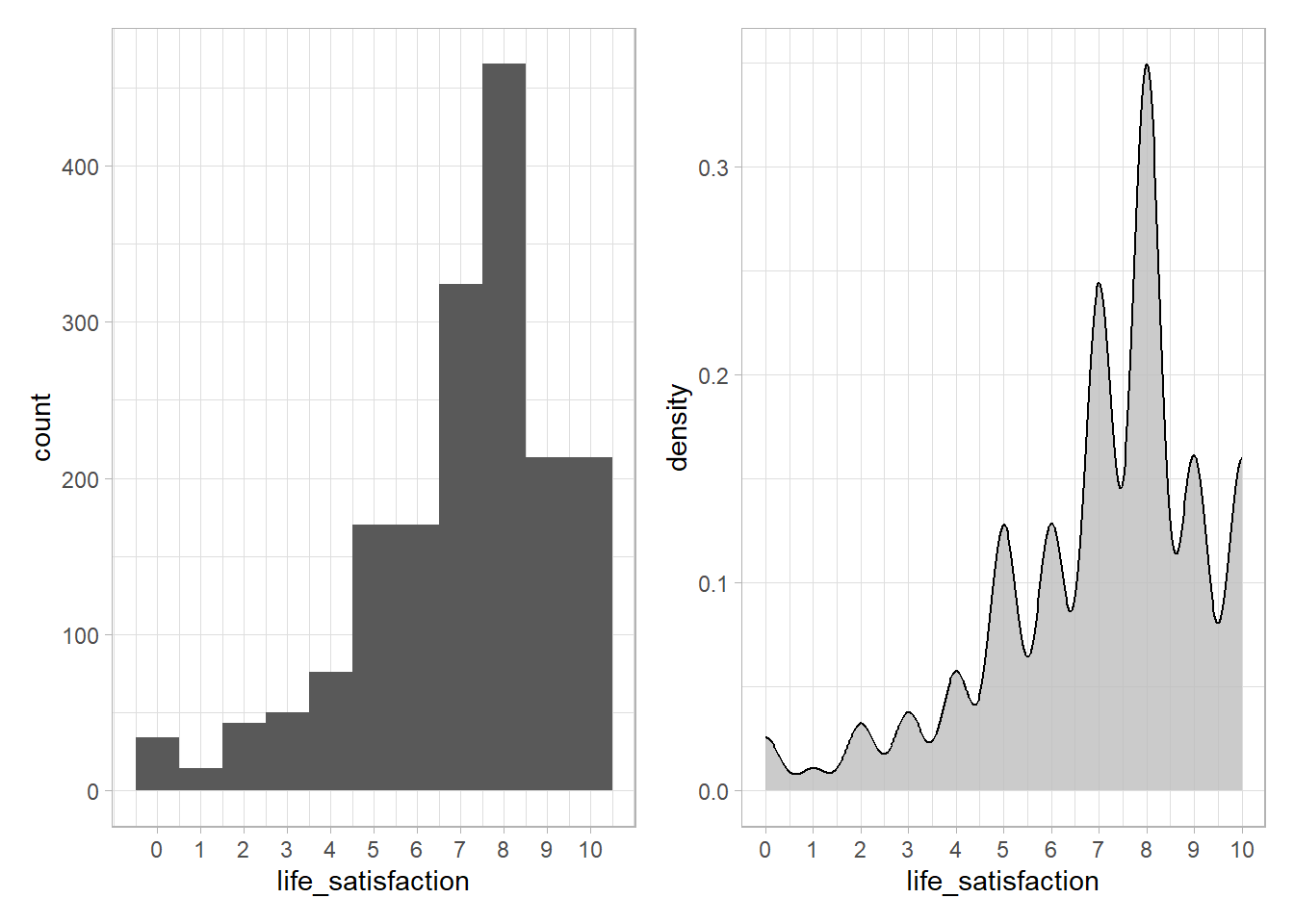
Insights
- For the visualization make sure to adapt scales to outcome variable. Also, play around with binwidth and bandwidth arguments to fully grasp distribution (see another example below).
- The mass of the distribution lies in the upper half, hence, we would expect any predictive model to predict those values for most individuals. There is less data on the lower values. Hence, any predictive model we built will also have less training data in this are to learn from which might result in worse predictions.
- With binary outcomes such graphs will also highlight potential imabalance, i.e., unequal sizes of the classes we want to predict.
# Missing value distribution
data %>%
select(where(~mean(is.na(.)) > 0.05)) %>% # select features with more than X % missing
plot_missing()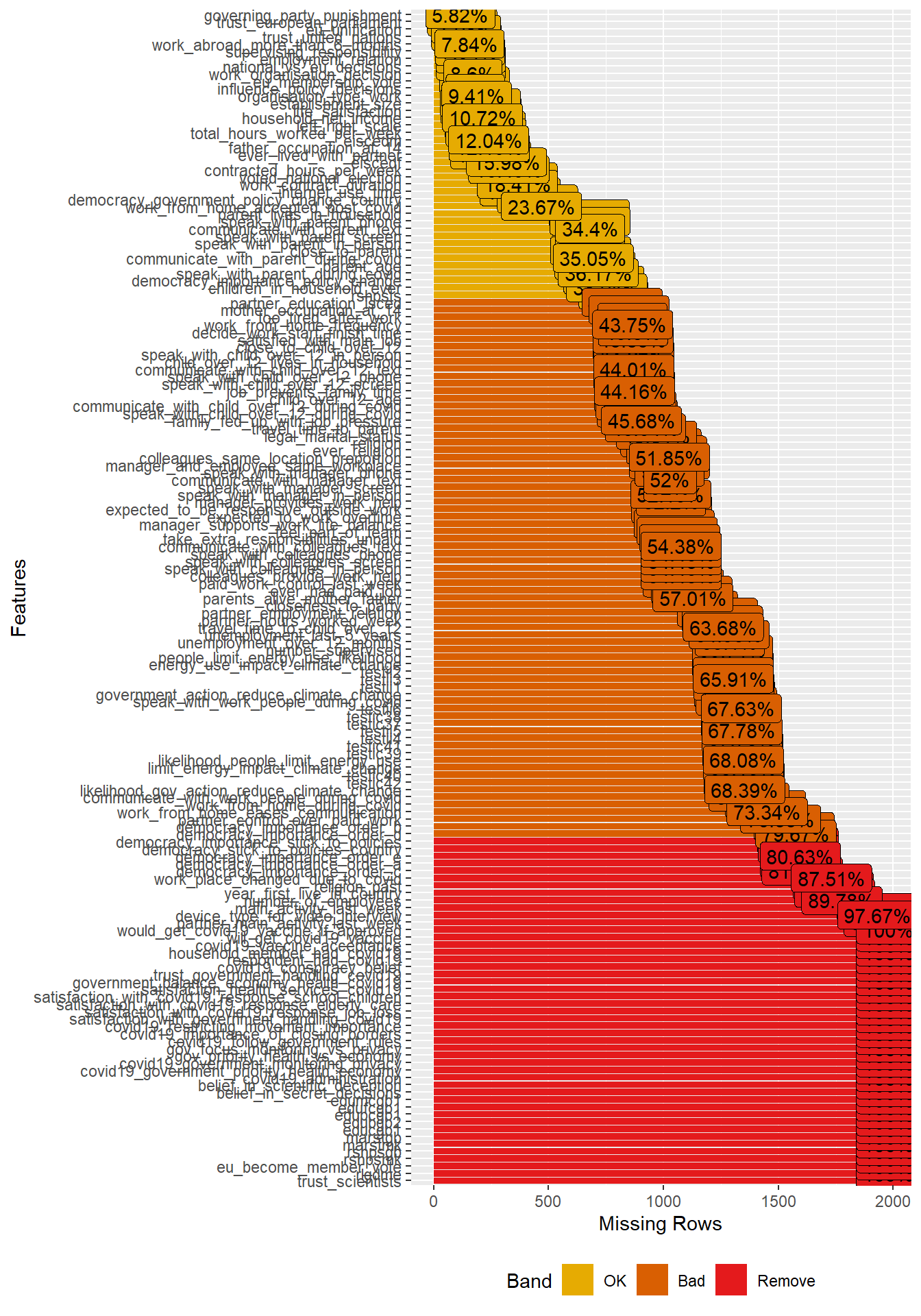
Insights
- Variables/features/predictors with a lot of missing data are generally not useful. Using them in our models would strongly decrease the size of our training data. Consider deleting them from the dataset or maybe imputing them.
- Also ask yourself why there are so many missing for some variables. Does it point to a bias of some kind or data errors?
# Missing value distribution
data %>%
select(where(~mean(is.na(.)) > 0.8)) %>% # select features with more than X % missing
plot_missing()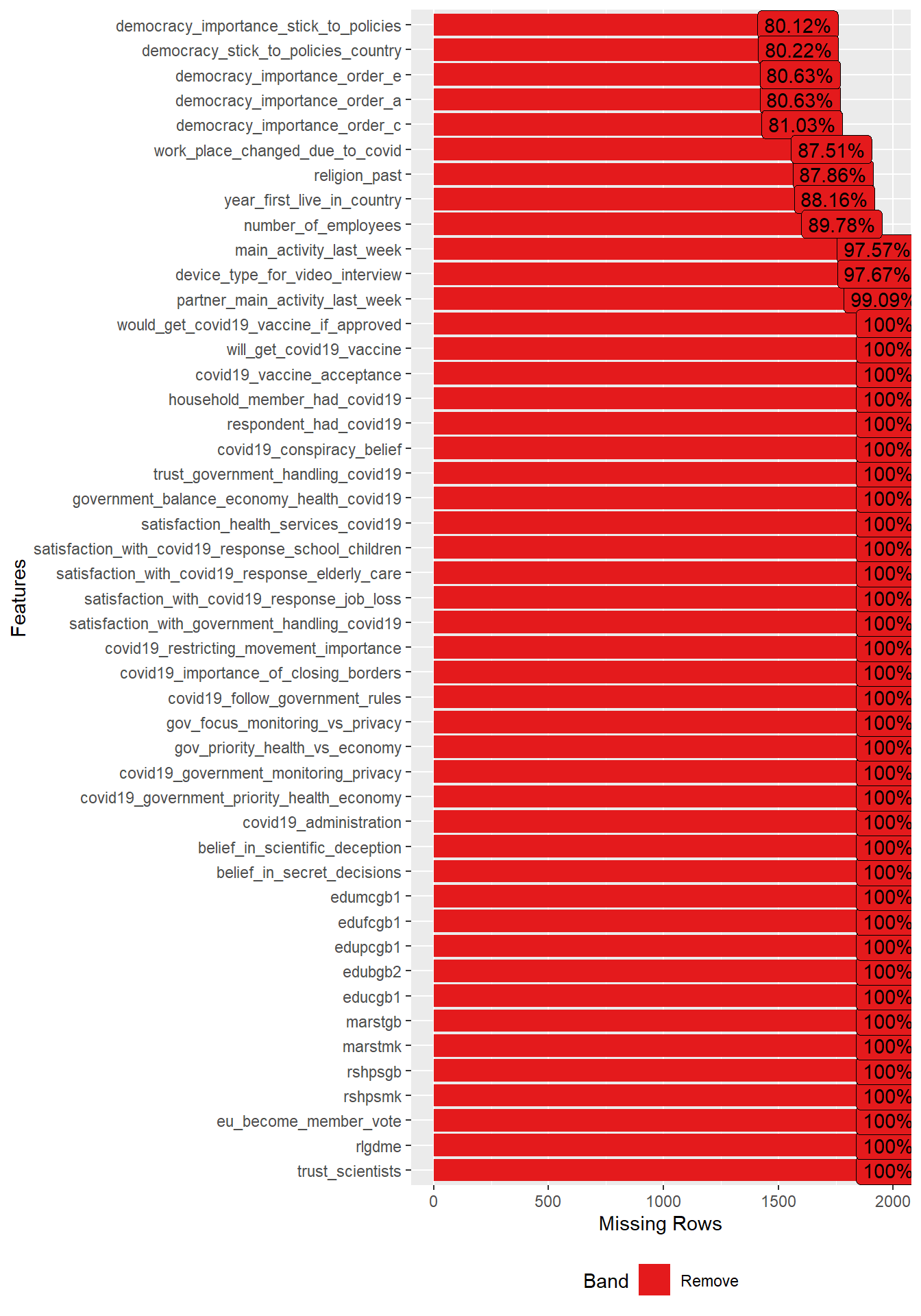
Insights
- Figure 5 would indicate if there is systematic missingness for certain variable types.
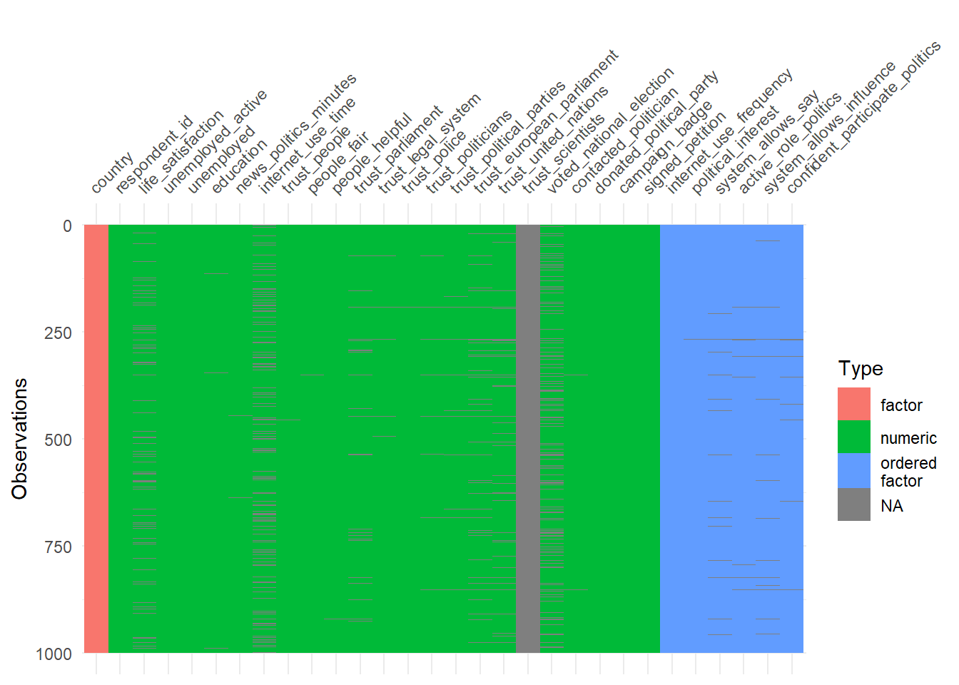
# Visualize the missings across variable types
vis_miss(data %>%
select(1:30) %>%
sample_n(1000),
sort_miss = TRUE) # try argument "cluster = TRUE" or "sort_miss = TRUE"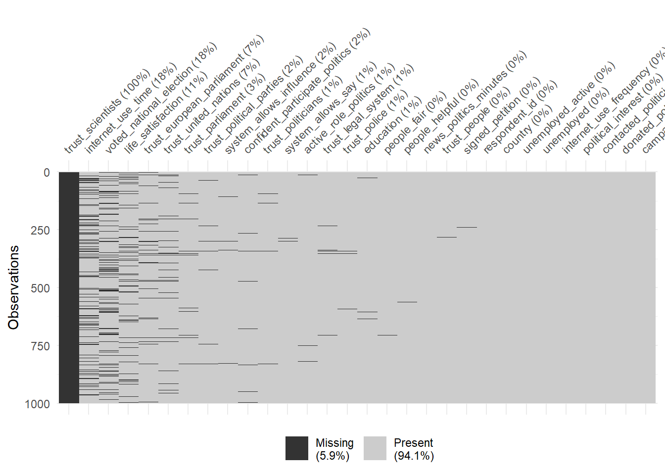
Insights
- The legend in Figure 6 shows the overall amount of missings. High values would be problematic as only few features could be sensibly be used for predictive modelling.
- For each variable we can also see the amount of missing on that variable.
- Also we don’t want to built a predictive (or explanatory) model that turn out to be based on very few data points, i.e., we should be the first to use that graph on our data.

Insights
- Figure 8 shows the number of observations across categorical variables.
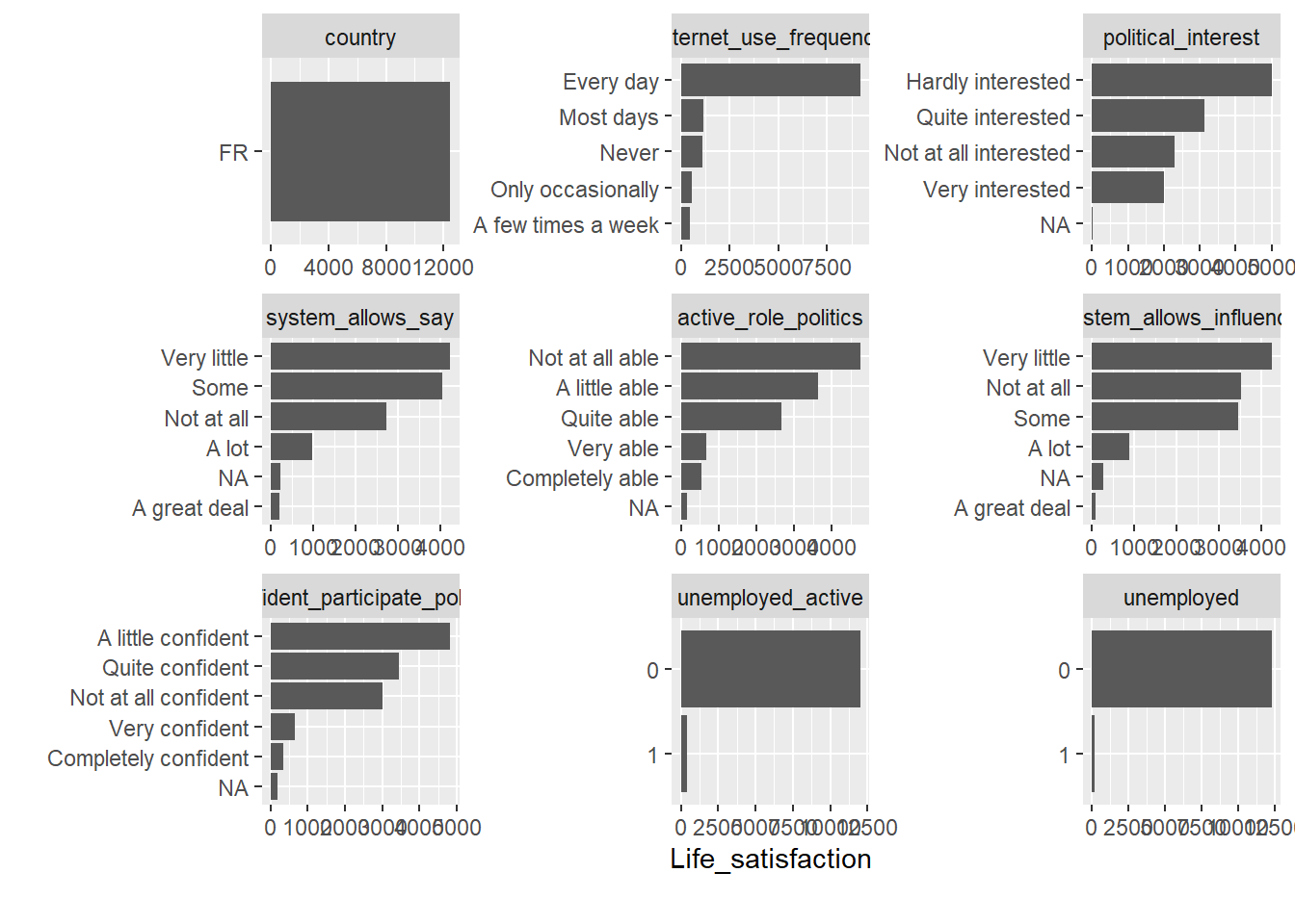
Insights
- Figure 8 shows the sum of our outcome variable across categories of other variables. Makes more sense for a categorical outcome (see below), less so for lifesatisfaction.
# Frequency distribution by a discrete variable
data %>%
mutate(female = as.factor(female)) %>% # dichotomize
select(female, country, political_interest, system_allows_say,
subjective_health, internet_use_frequency, unemployed) %>%
plot_bar(by = "female")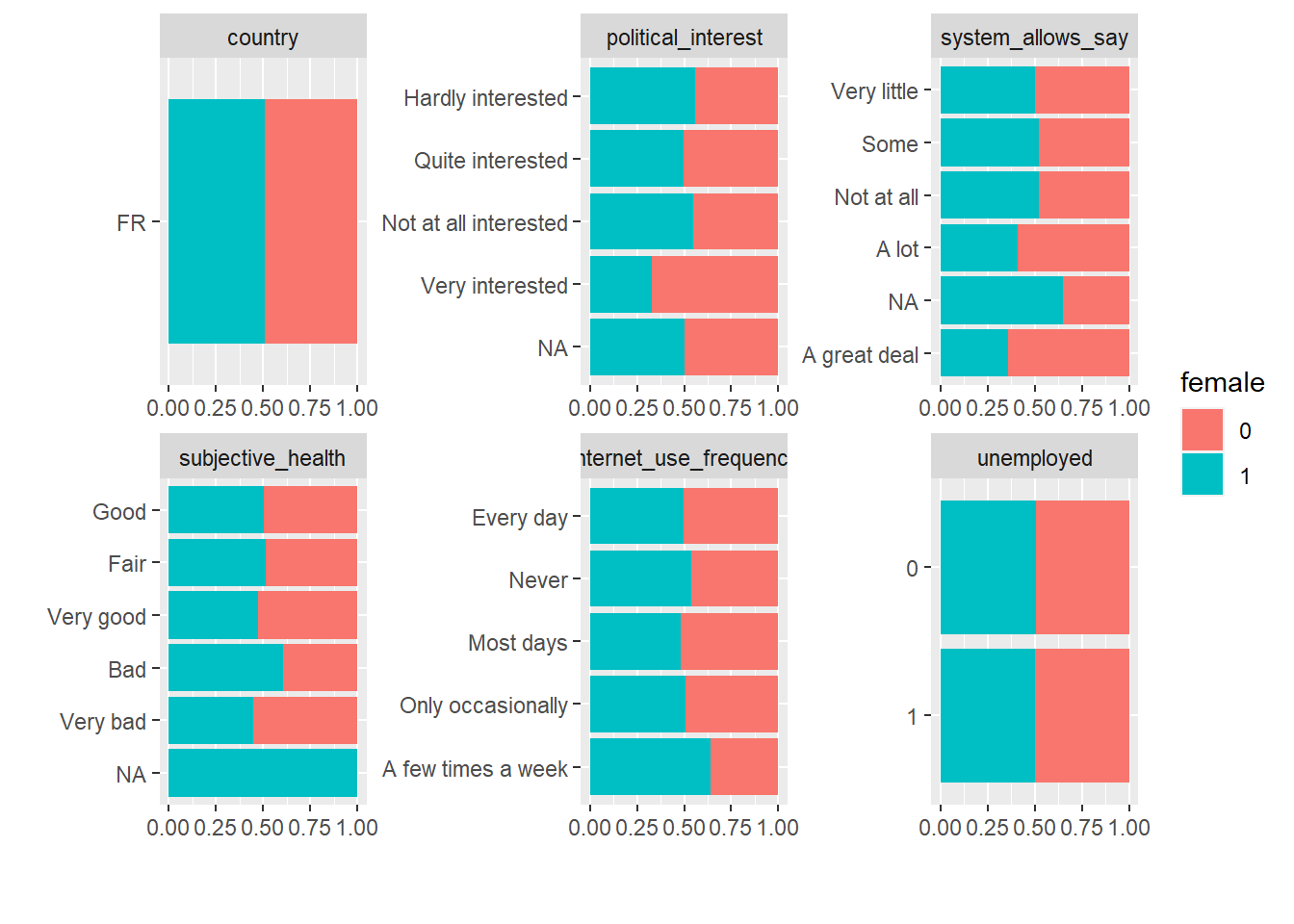
Insights
- Figure 9 is helpful to discover any systematic pattern between (categorical) socio-demographics.
## View estimated density distribution of continuous variables
data %>%
select(1:35) %>%
plot_density()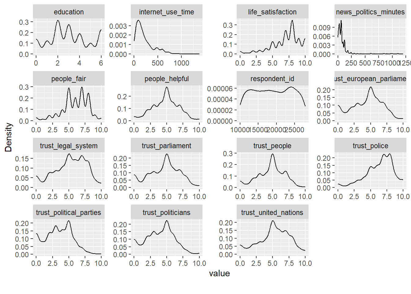
# View quantile-quantile plot of continuous variables
data %>%
sample_n(500) %>%
select(1:11) %>%
plot_qq()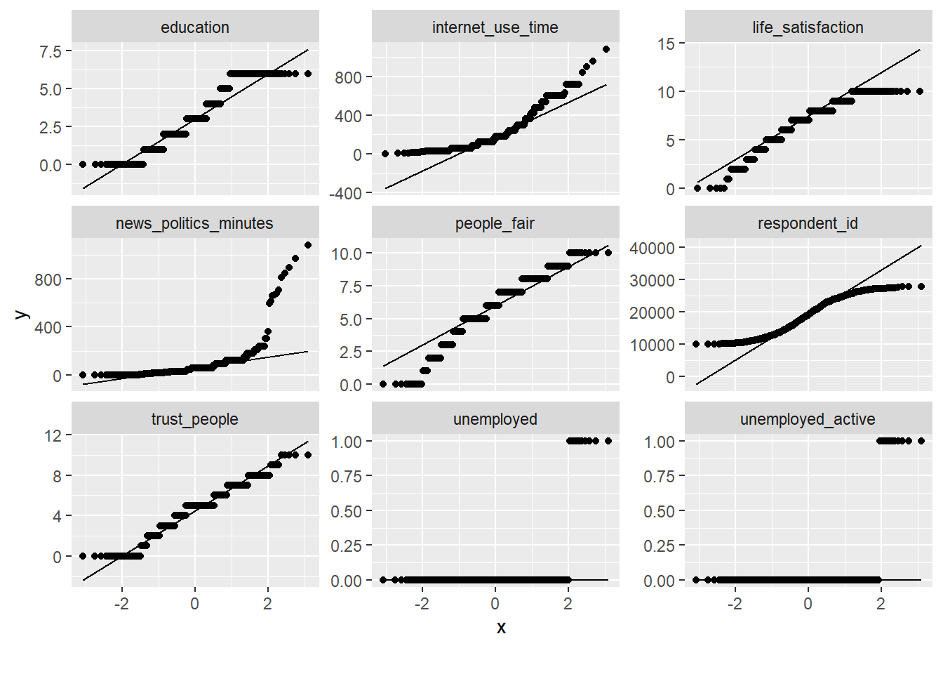
Insights
- Figure 12 A quantile-quantile plot (Q-Q plot) compares two probability distributions by plotting their quantiles against each other, i.e, here to identify whether contninous variables are far from a normal distribution. Values on the line indicate a normal distribution, deviations indicate deviations, e.g.,
new_politics_minuteshas some outliers deviating from the normal distribution as visible in Figure 11. Using a random sample my speed up computing the plot but should keep the same distribution.
# Quantile-quantile plot of continuous variables by discrete variable
data %>%
select(1:10) %>%
plot_qq(by = "internet_use_frequency")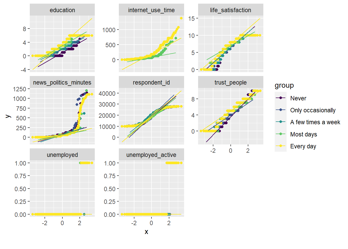
Insights
- Figure 13 shows Q-Q plots across continuous variables for subsets of a categorical variable. The aim is to identify whether continuous variable deviates from the normal distribution for certain subsets in our data (define by the categorical variable). Potentially, we could identify which subset category is responsible for the deviation from the normal variable (no clear pattersn in Figure 13).
# Overall correlation heatmap
data %>%
select(life_satisfaction, education, age, female, subjective_health) %>%
plot_correlation(cor_args = list("use" = "pairwise.complete.obs"))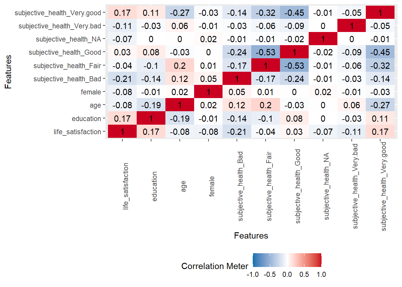
Insights
- Figure 14 may indicate any important predictors reflected by a stronger correlations.
# Bivariate continuous distributions based on cutting life_satisfaction
data %>%
select(1:22) %>%
plot_boxplot(by = "life_satisfaction")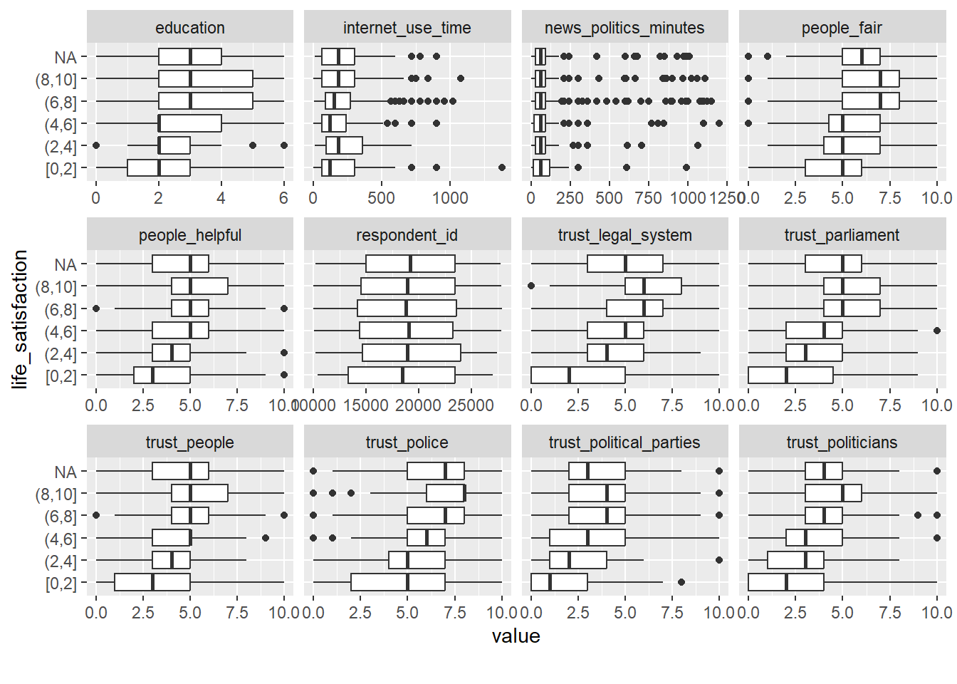
Insights
- Figure 15 discretizes our outcome variable and shows how it changes across values of other variables. If other variables strongly vary across our categorized outcome
life_satisfactionit may indicate that they have predictive power. Figure 15 shows that there is not meaningful variation forrespondent_idwhich makes sense since the id variable does not carry any information.
# Scatterplot `life_satisfaction` with other continuous features
data %>%
sample_n(500) %>%
select(1:12) %>%
split_columns %>% # split according to variable type
pluck(2) %>% # take numeric variables
plot_scatterplot(by = "life_satisfaction",
geom_point_args = list(alpha = 0.1, size = 1),
geom_jitter_args =
list(width = 0.3, height = 0.3),
ggtheme = theme_light())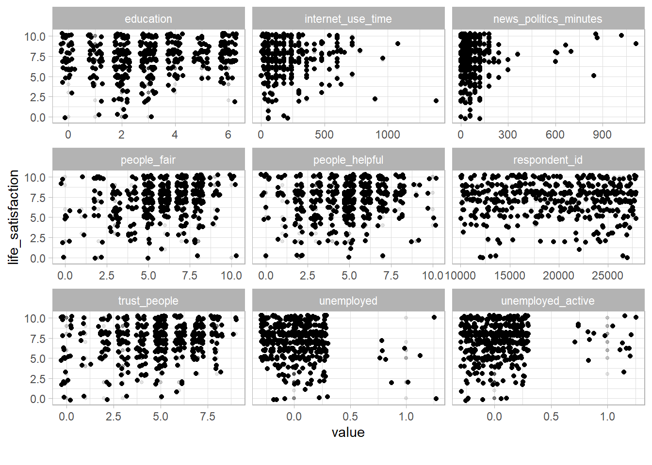
Insights
- Figure 16 provides an overview of the joint distribution of our outcome with other variables. It may help in discovering areas where we don’t have data in those joint distributions.
5 Exercise: Exploring a dataset (COMPASS data)
Overview of Compas dataset variables
id: ID of prisoner, numericname: Name of prisoner, factorcompas_screening_date: Date of compass screening, datedecile_score: the decile of the COMPAS score, numericis_recid: whether somone reoffended/recidivated (=1) or not (=0), numericis_recid_factor: same but factor variableage: a continuous variable containing the age (in years) of the person, numericage_cat: age categorizedpriors_count: number of prior crimes committed, numericsex: gender with levels “Female” and “Male”, factorrace: race of the person, factorjuv_fel_count: number of juvenile felonies, numericjuv_misd_count: number of juvenile misdemeanors, numericjuv_other_count: number of prior juvenile convictions that are not considered either felonies or misdemeanors, numeric
- To introduce classfication we are using a second data set on prisoners to predict whether they reoffend or not (recidivism). The data is based on a software that scores prisoners regarding their probability of reoffending/recidivating and whether they actually reoffended (Variable:
is_recid/is_recid_factorwhere 1 = yes, 0 = no). Please import this dataset calleddata(see code below.). - Then install and load the following packages:
skimr,modelsummary,DataExplorer,visdat,tidyverseandpatchwork(see code below.).
- Start by generating a few descriptive statistics to better understand the data. Use the
skim()function from the skimr package to get a first overview. What kind of variables does the data include? What interesting aspects stand out? - Use
datasummary_skim(..., type = "numeric")from themodelsummarypackage to produce some nice tables for both numeric and categorical variables. - Use
plot_intro()(Package:DataExplorer) to get a broad overview of the data. Is there anything particular about the dataset? - Missings determine success and failure of predictive models. Use the the functions
plot_missing()(Package:DataExplorer) andvis_miss()(Package:vis_datand usesort_miss = TRUE) to visualize missings. What stands out? - Special attention should be given to the outcome we want to predict. Explore the outcome using
table(..., useNA = "always")and graphs. Is there anything particular about it? - Finally,please use functions such as
plot_bar(),plot_histogram(),plot_density(),plot_qq(),plot_correlation()andplot_boxplot()to explore the data and whether certain predictors stand out in relation tois_recid. Since, the dataset is small you can simply apply those functions to the full dataset. What do you find?
Solutions
# 3.
# Summary statistics
#skim(data)
# 4.
datasummary_skim(data, type = "numeric")
datasummary_skim(data, type = "categorical")
# 5.
# Overview of data
plot_intro(data)
# 6.
# Visualize missings
plot_missing(data)
vis_miss(data, sort_miss = TRUE)
# 7.
##
table(data$is_recid, useNA = "always")
data %>%
ggplot(aes(x = is_recid)) +
geom_histogram(binwidth = 1) +
scale_x_continuous(breaks = 0:1) +
theme_light()
# 8.
## Frequency distribution of discrete variables
data %>% plot_bar()
## Distribution across discrete variables
data %>% plot_bar(with = "is_recid")
## View frequency distribution by a discrete variable
data %>% plot_bar(by = "is_recid_factor")
## View histogram of continuous variables
data %>% plot_histogram()
## View estimated density distribution of continuous variables
data %>% plot_density()
## View quantile-quantile plot of continuous variables
data %>%
sample_n(1000) %>%
plot_qq()
## View quantile-quantile plot of continuous variables by feature `is_recid`
data %>%
sample_n(1000) %>%
plot_qq(by = "is_recid")
## View overcorrelation heatmap
data %>%
plot_correlation(cor_args = list("use" = "pairwise.complete.obs"))
## View bivariate continuous distribution based on `cut`
data %>%
plot_boxplot(by = "is_recid")6 All the code
# install.packages(pacman)
pacman::p_load(tidyverse,
               tidymodels,
               knitr,
               kableExtra,
               DataExplorer,
               visdat)
# Load the .RData file into R
load(url(sprintf("https://docs.google.com/uc?id=%s&export=download",
                         "173VVsu9TZAxsCF_xzBxsxiDQMVc_DdqS")))
library(skimr)
library(modelsummary)

# Data overview
# skim(data) # Run this in R (output is too long)
datasummary_skim(data, type = "numeric")
datasummary_skim(data %>% select(1:50), type = "categorical")
library(ggplot2)
library(patchwork)
p1 <- ggplot(data = data, aes(x = life_satisfaction)) +
  geom_histogram(binwidth = 1) +
  scale_x_continuous(breaks = 0:10) +
  theme_light()
p2 <- ggplot(data = data, aes(x = life_satisfaction)) +
  geom_density(fill="gray", alpha=0.8) + # try bw = 0.4
  scale_x_continuous(breaks = 0:10) +
  theme_light()
p1+p2
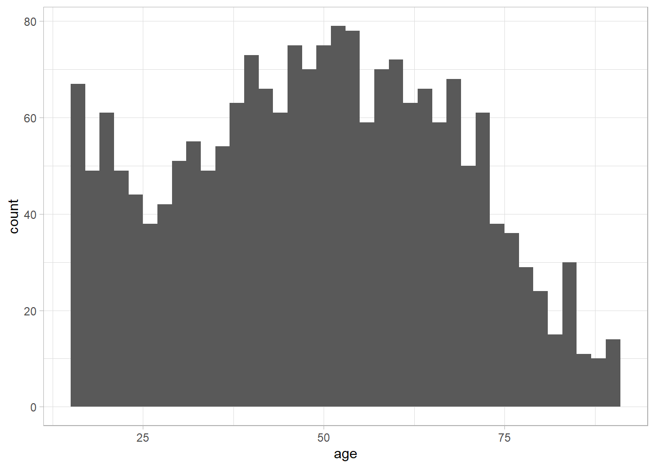
# Try playing around with variable age
ggplot(data = data, aes(x = age)) +
  geom_histogram(binwidth = 2) +
  theme_light()
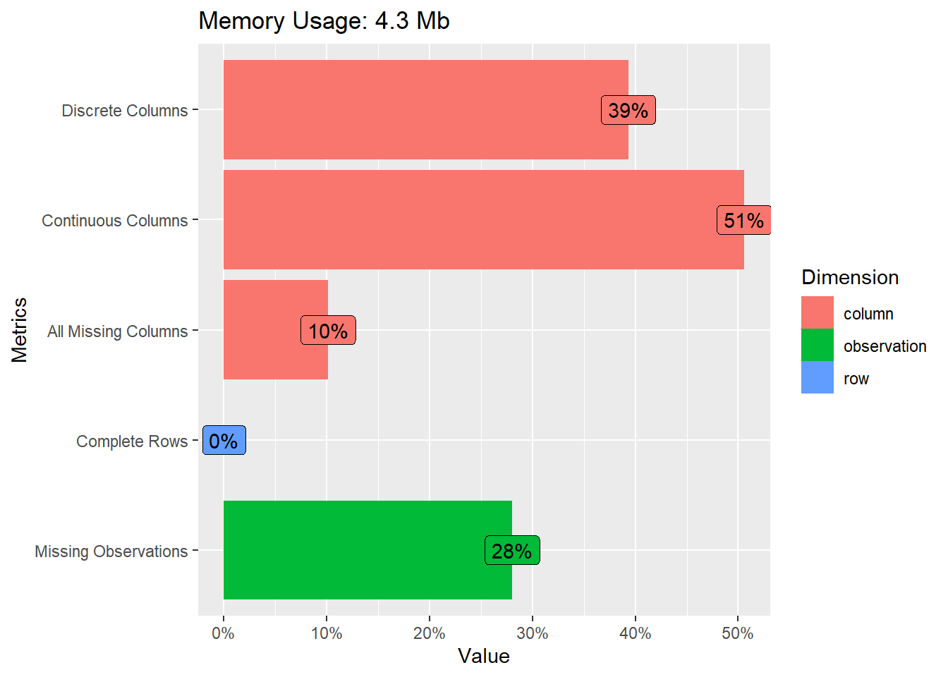
library(DataExplorer)
library(visdat)
# Overview of dataset
plot_intro(data)
# Missing value distribution
data %>%
  select(where(~mean(is.na(.)) > 0.05)) %>% # select features with more than X % missing
    plot_missing()
# Missing value distribution
data %>%
  select(where(~mean(is.na(.)) > 0.8)) %>% # select features with more than X % missing
    plot_missing()
# View missings across variables
vis_dat(data %>%
          select(1:30) %>%
           sample_n(1000))
# Visualize the missings across variable types
vis_miss(data %>%
           select(1:30) %>%
           sample_n(1000),
           sort_miss = TRUE) # try argument "cluster = TRUE" or "sort_miss = TRUE"
# Frequency distribution of discrete variables
data %>%
  select(1:20) %>%
    plot_bar()
data %>%
  select(1:20) %>%
    plot_bar(with = "life_satisfaction")
# Frequency distribution by a discrete variable
data %>%
  mutate(female = as.factor(female)) %>% # dichotomize
  select(female, country, political_interest, system_allows_say,
         subjective_health, internet_use_frequency, unemployed) %>%
          plot_bar(by = "female")
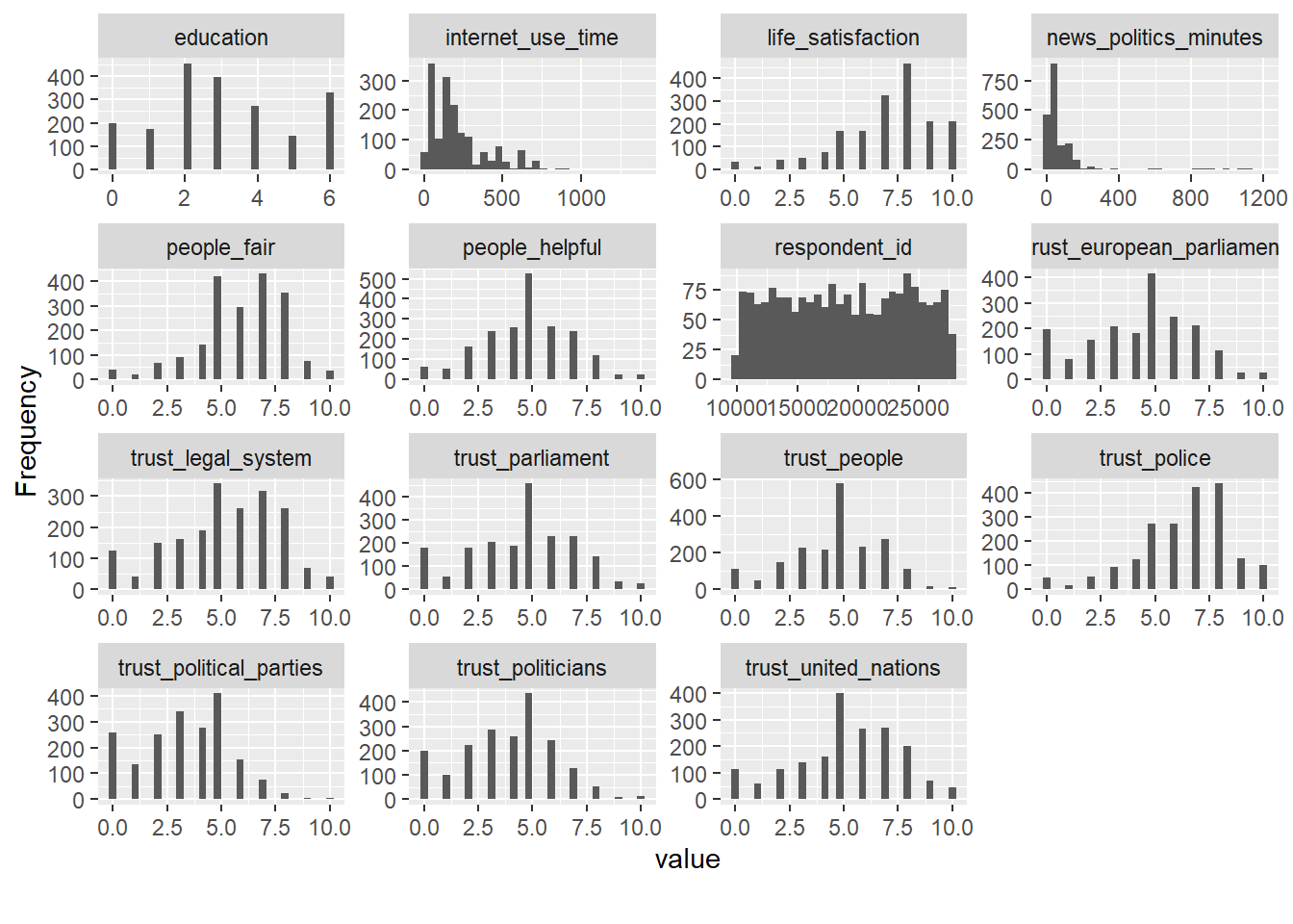
# View histogram of continuous variables
data %>%
  select(1:30) %>%
      plot_histogram()
## View estimated density distribution of continuous variables
data %>%
  select(1:35) %>%
    plot_density()
# View quantile-quantile plot of continuous variables
data %>%
  sample_n(500) %>%
  select(1:11) %>%
    plot_qq()
# Quantile-quantile plot of continuous variables by discrete variable
data %>%
  select(1:10) %>%
  plot_qq(by = "internet_use_frequency")
# Overall correlation heatmap
data %>%
  select(life_satisfaction, education, age, female, subjective_health) %>%
      plot_correlation(cor_args = list("use" = "pairwise.complete.obs"))
# Bivariate continuous distributions based on cutting life_satisfaction
data %>%
  select(1:22) %>%
      plot_boxplot(by = "life_satisfaction")
# Scatterplot `life_satisfaction` with other continuous features
data %>%
  sample_n(500) %>%
  select(1:12) %>%
      split_columns %>% # split according to variable type
        pluck(2) %>% # take numeric variables
            plot_scatterplot(by = "life_satisfaction",
                             geom_point_args = list(alpha = 0.1, size = 1),
                             geom_jitter_args =
                               list(width = 0.3, height = 0.3),
ggtheme = theme_light())Footnotes
I added some missings on the life satisfaction variable!↩︎