Tuning models
Learning outcomes/objective: Learn…
- …what tuning means.
- …how to tune models using tidymodels.
- …how to tune a random forest/a ridge regression/a lasso.
Source(s): Closely based on superbe summary in Arnold et al. (2024) (check out their research); Tune model parameters
1 Why care about hyperparameters?
- Aim of ML: Find a model that generalizes well from training data to new, unseen data
- Reminder: We evaluate the model using unseen test data, and then usually want to predict outcomes of further unseen data
- Hyperparameter determine a model’s capacity to generalize and may critically affect a model’s performance
- Arnold et al. (2024, 1) find that among 64 machine learning-related political science papers1…
- 36 publications (56.25 %) do not report the values of their hyper- parameters
- 49 publications (76.56 %) do not share information their usage of tuning to find good hyperparameters
- 13 publications (20.31 %) offer a complete account of hyperparameters/tuning
2 What are hyperparameters and why do they need to be tuned? (1)
- Many machine learning models have parameters and also hyperparameters
- Model parameters are learned during training
- Hyperparameters typically set before training
- Determine what a model can learn and how well the model will perform on out-of-sample data (set at meta-level)
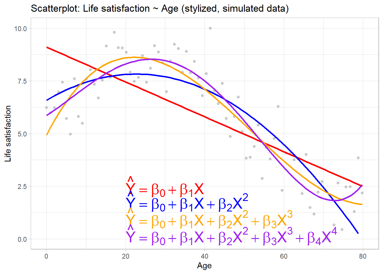
- Consider stylized example in Figure 1
- Linear regression approach could model relationship between \(X\) and \(Y\) as \(\hat{Y}=\beta_{0} + \beta_{1}X\)
- More flexible model would include additional polynomials in X
- Choosing \(\lambda=2\) \(\rightarrow\) belief that \(Y\) is best predicted by a quadratic function of \(X\), i.e., \(\hat{Y}=\beta_{0} + \beta_{1}X + \beta_{2}X^{2}\)
- But we could also rely on data to find optimal value of \(\lambda\)
- Estimate models with different \(\lambda\)’s, evaluate accuracy using MSE and pick best \(\lambda\)
3 What are hyperparameters and why do they need to be tuned? (2)
- Polynomial regression comes with both parameters and hyperparameters
- Parameters are variables that belong to the model itself (here regression coefficients)
- Hyperparameters are variables that help specify exact model
- Here the hyperparameter \(\lambda\) determines how many parameters (\(\beta\)s) are learned
- Anything part of the function that maps the data to a performance measure and that can be set to different values can be considered a hyperparameter, e.g., number of trees in a random forest
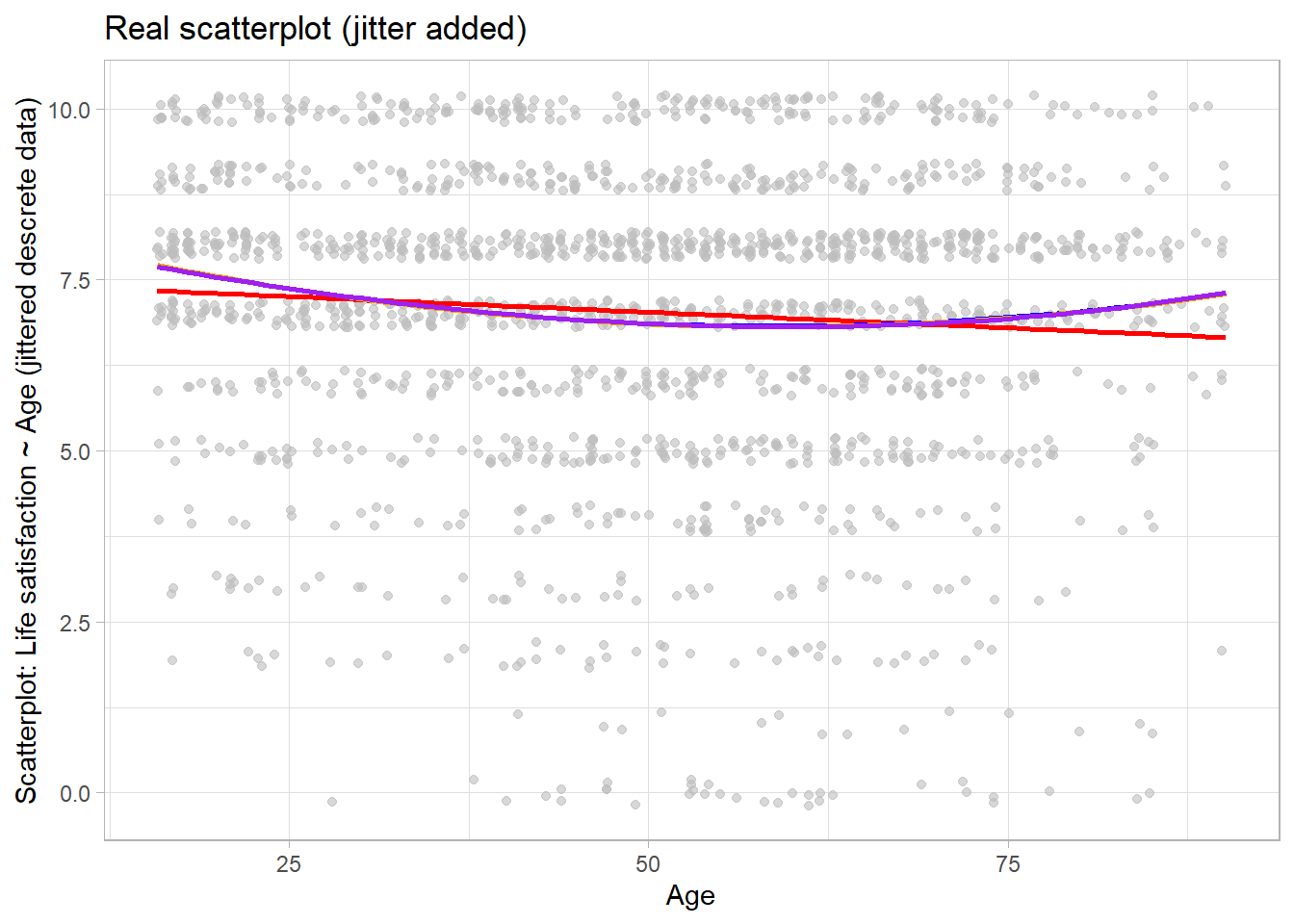
4 The “real” Age-Life satisfaction relationship
Figure 2 illustrates that real relationships seldom follow the nice shape depicted in Figure 1.
5 Steps in tuning (Arnold et al. 2024)
- Understanding the model: What are the available hyperparameters? How do they affect the model?
- Choosing a performance measure: What is a good performance for the machine learning model? (e.g., MSE, MAE, F-1)
- Defining a sensible search space:
- Useful starting points: hyperparameter default values in software libraries, recommendations from the literature, or own previous experience
- Finding the best combination in the search space:
- Grid search: try every possible combination of hyperparameters of the search space to find optimal combination
- Random search: each run picks a different random set of hyperparameters from the search space
- Tuning under strong resource constraints: . If the model training is too involved, adaptive approaches such as sequential model-based Bayesian optimization allow for efficiently identifying and testing promising hyperparameter candidates.
- Important!!!: Describe whether/how hyperparameters were tuned and what final value were chosen in main body/appendix of paper
6 Models and their hyperparameters
6.1 Lasso & ridge regression
- See
?details_linear_reg_glmnetfor details forglmnetpackage - These models have 2 tuning parameters
penalty: Amount of Regularization (default: see below)2- The
penaltyparameter has no default and requires a single numeric value
- The
mixture: Proportion of Lasso Penalty (default: 1)- A value of
mixture = 1corresponds to a pure lasso model, whilemixture = 0indicates ridge regression
- A value of
6.2 Random forest
- See
?details_rand_forest_rangerfor details forrangerpackage - Can be used for both classification and regression
# = number of- Model has 8 tuning (hyper-)parameters
mtry: # Randomly Selected Predictors (default: depends on number of columns)trees: # Trees (default: 500)min_n: Minimal Node Sizemin_ndefault depends on the mode. For regression, a value of 5 is the default. For classification, a value of 10 is used.
6.3 XGBoost tuning parameters
- See
?details_boost_tree_xgboostfor details forxgboostpackage - Can be used for both classification and regression
# = number of- Model has 8 tuning (hyper-)parameters
tree_depth: Tree depth (default: 6)3trees: # trees (default: 15)4learn_rate: Learning rate (default: 0.3)5- Picking lower value might be better but is slower
mtry: # randomly selected predictors among which splitting candidate is picked (default: see below)min_n: Minimal node size before stopping splitting (default: 1)loss_reduction: Minimum loss reduction (default: 0.0)6sample_size: Proportion observations sampled (default: 1.0)7stop_iter: # iterations before stopping (default: Inf)8
7 Lab: Tuning a random forest
Here, we will simply re-use Step 1 and Step 2 from the corresponding random forest lab.
# Extract data with missing outcome
  data_missing_outcome <- data %>% filter(is.na(life_satisfaction))
  dim(data_missing_outcome)
[1] 0 7# Omit individuals with missing outcome from data
data <- data %>% drop_na(life_satisfaction) # ?drop_na
dim(data)[1] 1760 7# STEP 2
# Split the data into training and test data
data_split <- initial_split(data, prop = 0.80)
data_split # Inspect<Training/Testing/Total>
<1408/352/1760> # Extract the two datasets
data_train <- training(data_split)
data_test <- testing(data_split) # Do not touch until the end!
# Create resampled partitions
set.seed(345)
data_folds <- vfold_cv(data_train, v = 2) # V-fold/k-fold cross-validation
data_folds # data_folds now contains several resamples of our training data # 2-fold cross-validation
# A tibble: 2 × 2
splits id
<list> <chr>
1 <split [704/704]> Fold1
2 <split [704/704]> Fold27.1 Step 3: Specify recipe, model, workflow and tuning parameters
Similar to ridge or lasso regression a random forest has parameters that we can try to tune. Below, we create a model specification for a RF where we will tune…
mtrythe number of predictors to sample at each split andmin_nthe number of observations needed in each resulting node to keep splitting.
Insights: What is mtry and min_n?
- Number of Predictors to Sample at Each Split (
mtry): This hyperparameter controls the number of predictors randomly sampled at each split in the decision tree building process. A smaller value ofmtrycan lead to less correlation between individual trees in the forest, potentially reducing overfitting, but it may also increase the randomness in the model. Conversely, a larger value ofmtrycan lead to stronger individual trees but might increase the risk of overfitting. Typically, you can try different values ofmtryand choose the one that provides the best performance based on cross-validation or other evaluation methods. - Minimum Number of Observations in Each Node (
min_n): This hyperparameter determines the minimum number of observations required in a node for it to be eligible for further splitting. If a node has fewer thanmin_nobservations, it won’t be split further, effectively controlling the depth and complexity of the trees. Setting a higher value ofmin_ncan help prevent overfitting by creating simpler trees, but it may also lead to underfittingif set too high.
These are hyperparameters that can’t be learned from data when training the model. (cf. Source)
  # Define recipe
  model_recipe <-
    recipe(formula = life_satisfaction ~ ., data = data_train) %>%
    step_naomit(life_satisfaction, all_predictors()) %>% # better deal with missings beforehand
    step_nzv(all_predictors(), freq_cut = 0, unique_cut = 0) %>% # remove variables with zero variances
    step_novel(all_nominal_predictors()) %>% # prepares data to handle previously unseen factor levels
    #step_unknown(all_nominal_predictors()) %>% # categorizes missing categorical data (NA's) as `unknown`
    step_dummy(all_nominal_predictors(), -has_role("id vars")) %>% # dummy codes categorical variables
    step_zv(all_predictors()) %>% # remove vars with only single value
    step_normalize(all_predictors()) # normale predictors

  # Inspect the recipe
    model_recipe


# Specify model with tuning
model1 <- rand_forest(
  mtry = tune(), # tune mtry parameter (number of predictors to sample at each split)
  trees = 1000, # grow 1000 trees
  min_n = tune() # tune min_n parameter (min N in Node to split)
) %>%
  set_mode("regression") %>%
  set_engine("ranger",
             importance = "permutation") # potentially computational intensive


# Specify workflow (with tuning)
workflow1 <- workflow() %>%
  add_recipe(model_recipe) %>%
  add_model(model1)
7.2 Step 4: Tune, evaluate the model using resampling and choose/explore the best model
7.2.1 Tune, evaluate the model using resampling
Below we use tune_grid() to compute performance metrics (e.g. accuracy or RMSE) for pre-defined set of tuning parameters that correspond to a model or recipe across one or more resamples of the data (below 10 stored in data_folds).
# Specify to use parallel processing
doParallel::registerDoParallel()

set.seed(345)
tune_result <- tune_grid(
  workflow1,
  resamples = data_folds,
  grid = 10 # choose 10 grid points automatically
)

tune_result
# Tuning results
# 2-fold cross-validation
# A tibble: 2 × 4
splits id .metrics .notes
<list> <chr> <list> <list>
1 <split [704/704]> Fold1 <tibble [20 × 6]> <tibble [0 × 3]>
2 <split [704/704]> Fold2 <tibble [20 × 6]> <tibble [0 × 3]>
Visualizing the results helps us to evaluate the tuning results. Figure 3 indicates that higher values of min_n and lower values of mtry seem to work better in terms of accuracy.
tune_result %>%
  collect_metrics() %>% # extract metrics
  filter(.metric == "rmse") %>% # keep rmse only
  select(mean, min_n, mtry) %>% # subset variables
  pivot_longer(min_n:mtry, # convert to longer
    values_to = "value",
    names_to = "parameter"
  ) %>%
  ggplot(aes(value, mean, color = parameter)) + # plot!
  geom_point(show.legend = FALSE) +
  facet_wrap(~parameter, scales = "free_x") +
  labs(x = NULL, y = "RMSE")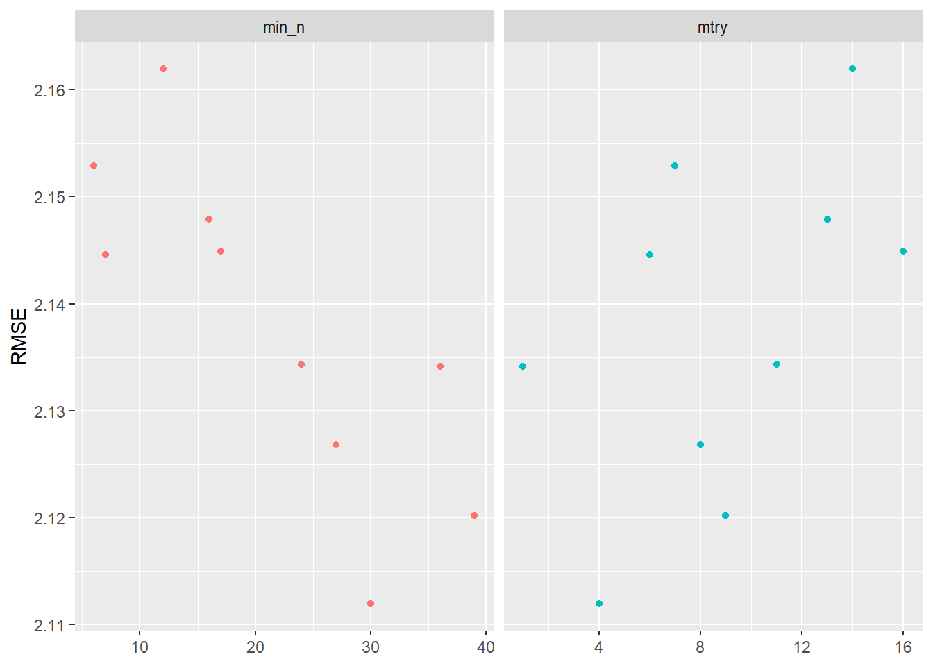
After getting this first glimpse in Figure 3 we might want to make further changes to the grid values that we use for tuning. Below we pick ranges that turned out to be better in Figure 3:
grid1 <- grid_regular(
  mtry(range = c(0, 10)), # define range for mtry
  min_n(range = c(20, 40)), # define range for min_n
  levels = 6 # number of values of each parameter to use to make the regular grid
)

grid1
# A tibble: 36 × 2
mtry min_n
<int> <int>
1 0 20
2 2 20
3 4 20
4 6 20
5 8 20
6 10 20
7 0 24
8 2 24
9 4 24
10 6 24
# ℹ 26 more rowsThen we re-do the tuning using those values:
set.seed(456)
tune_result2 <- tune_grid(
  workflow1,
  resamples = data_folds,
  grid = grid1
)

tune_result2
# Tuning results
# 2-fold cross-validation
# A tibble: 2 × 4
splits id .metrics .notes
<list> <chr> <list> <list>
1 <split [704/704]> Fold1 <tibble [72 × 6]> <tibble [0 × 3]>
2 <split [704/704]> Fold2 <tibble [72 × 6]> <tibble [0 × 3]>Again we visualize the results in Figure 4:
tune_result2 %>%
  collect_metrics() %>%
  filter(.metric == "rmse") %>%
  select(mean, min_n, mtry) %>%
  pivot_longer(min_n:mtry,
    values_to = "value",
    names_to = "parameter"
  ) %>%
  ggplot(aes(value, mean, color = parameter)) +
  geom_point(show.legend = FALSE) +
  facet_wrap(~parameter, scales = "free_x") +
  labs(x = NULL, y = "RMSE")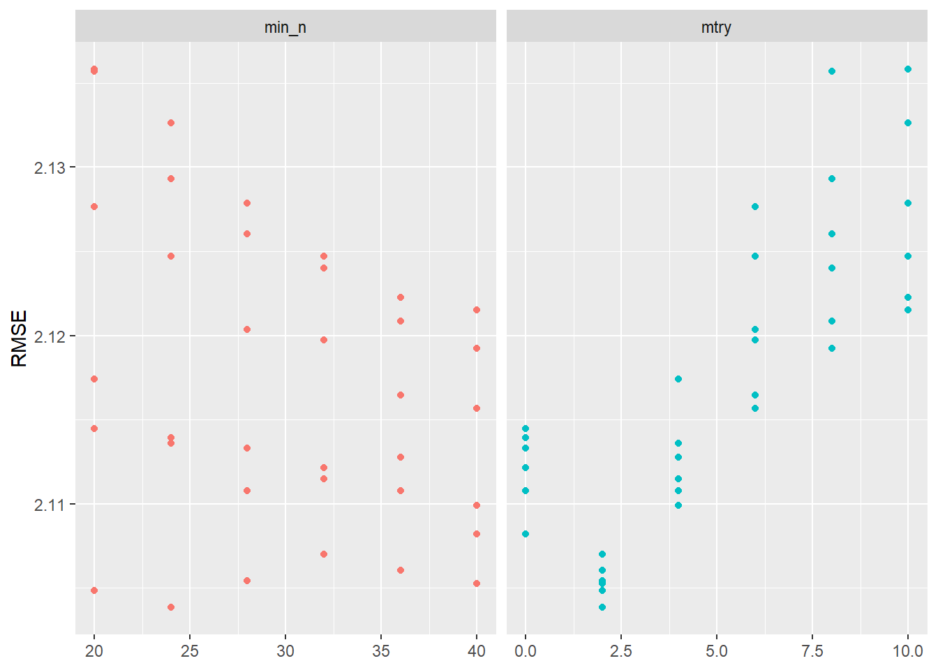
7.2.2 Choose best model after tuning
Choosing the best model, i.e., the model with the best parameter choices obtained in the tuning above (tune_result2), can be done with the select_best() function. After having selected the best parameter values, we update our original model specification stored in model1 using the finalize_model() function.
7.3 Step 5: Fit final model to training data and assess accuracy
Once we are happy with our tuned random forest model and have chosen the best model specification stored in model_final we can fit our workflow to the training data data_train again and also assess it’s accuracy again.
# Define final workflow
workflow_final <- workflow() %>%
  add_recipe(model_recipe) %>% #  use standard recipe
  add_model(model_final) # use final model

# Fit final model
fit_final <- fit(workflow_final, data = data_train)
fit_final
══ Workflow [trained] ══════════════════════════════════════════════════════════
Preprocessor: Recipe
Model: rand_forest()
── Preprocessor ────────────────────────────────────────────────────────────────
6 Recipe Steps
• step_naomit()
• step_nzv()
• step_novel()
• step_dummy()
• step_zv()
• step_normalize()
── Model ───────────────────────────────────────────────────────────────────────
Ranger result
Call:
ranger::ranger(x = maybe_data_frame(x), y = y, mtry = min_cols(~2L, x), num.trees = ~1000, min.node.size = min_rows(~24L, x), importance = ~"permutation", num.threads = 1, verbose = FALSE, seed = sample.int(10^5, 1))
Type: Regression
Number of trees: 1000
Sample size: 1408
Number of independent variables: 17
Mtry: 2
Target node size: 24
Variable importance mode: permutation
Splitrule: variance
OOB prediction error (MSE): 4.38442
R squared (OOB): 0.1187971 # Q: What do the values for `mtry` and `min_n` in the final model mean?
# Check accuracy in training data using MAE
augment(fit_final, new_data = data_train) %>%
mae(truth = life_satisfaction, estimate = .pred)# A tibble: 1 × 3
.metric .estimator .estimate
<chr> <chr> <dbl>
1 mae standard 1.53
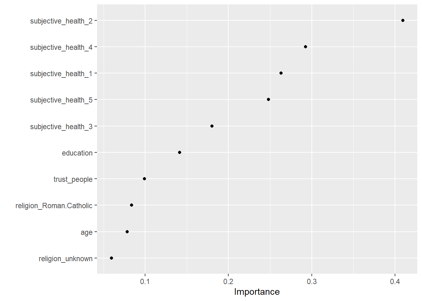
Now, that we have our final model we can also explore it assessing variable importance (i.e., which variables where the most relevant to find splits) using the vip package. We can use vi() and vip() to extract or extract+plot the variable importance of different predictors as shown in Table 1 and Figure 5. The vi() and vip() function does only like objects of class ranger, hence we have to directly access is in the layer object using fit_final$fit$fit$fit
# Visualize variable importance
# install.packages("vip")
library(vip)
fit_final$fit$fit %>%
    vip::vi() %>%
kable()| Variable | Importance |
|---|---|
| subjective_health_2 | 0.4092632 |
| subjective_health_4 | 0.2924986 |
| subjective_health_1 | 0.2630524 |
| subjective_health_5 | 0.2479773 |
| subjective_health_3 | 0.1800742 |
| education | 0.1414436 |
| trust_people | 0.0990111 |
| religion_Roman.Catholic | 0.0836794 |
| age | 0.0782775 |
| religion_unknown | 0.0595330 |
| unemployed | 0.0393121 |
| religion_Islam | 0.0292091 |
| religion_Other.Non.Christian.religions | 0.0076203 |
| religion_Eastern.religions | -0.0001497 |
| religion_Other.Christian.denomination | -0.0009572 |
| religion_Jewish | -0.0019350 |
| religion_Protestant | -0.0047955 |
7.4 Step 6: Fit final model to test data and assess accuracy
We then evaluate the accuracy of this model which is based on the training data using the test data data_test. We use augment() to obtain the predictions:
# A tibble: 352 × 8
   life_satisfaction unemployed trust_people education   age religion
               <dbl>      <dbl>        <dbl>     <dbl> <dbl> <fct>
 1                 6          0            0         4    51 unknown
 2                 7          0            7         6    50 unknown
 3                 7          0            1         0    46 unknown
 4                 8          0            5         0    74 Islam
 5                10          0            4         4    20 Roman Catholic
 6                 8          0            3         3    31 unknown
 7                 8          0            8         3    33 Roman Catholic
 8                 7          0            8         6    27 Roman Catholic
 9                 4          0            2         3    72 unknown
10                10          0            6         1    70 Roman Catholic
# ℹ 342 more rows
# ℹ 2 more variables: subjective_health <ord>, .pred <dbl>
And can directly pipe the result into functions such as rsq(), rmse() and mae() to obtain the corresponding measures of accuracy in the test data data_test.
# A tibble: 1 × 3
.metric .estimator .estimate
<chr> <chr> <dbl>
1 rsq standard 0.0865# A tibble: 1 × 3
.metric .estimator .estimate
<chr> <chr> <dbl>
1 rmse standard 2.10# A tibble: 1 × 3
.metric .estimator .estimate
<chr> <chr> <dbl>
1 mae standard 1.64The corresponding accuracy measures can now be compared to those of an untuned random forest model.
8 Lab: Tuning ridge regression
See earlier description here (right click and open in new tab).
We first import the data into R:
# Drop missings on outcome variable
data <- data %>%
drop_na(life_satisfaction) %>%
select(where(~mean(is.na(.)) < 0.1)) %>%
na.omit()
# Split the data into training and test data
data_split <- initial_split(data, prop = 0.80)
data_split # Inspect<Training/Testing/Total>
<696/174/870># Extract the two datasets
data_train <- training(data_split)
data_test <- testing(data_split) # Do not touch until the end!
# Create resampled partitions
set.seed(345)
data_folds <- vfold_cv(data_train, v = 2) # V-fold/k-fold cross-validation
data_folds # data_folds now contains several resamples of our training data # 2-fold cross-validation
# A tibble: 2 × 2
splits id
<list> <chr>
1 <split [348/348]> Fold1
2 <split [348/348]> Fold2 # You can also try loo_cv(data_train) instead
# Define recipe
recipe1 <-
recipe(formula = life_satisfaction ~ ., data = data_train) %>%
update_role(respondent_id, new_role = "ID") %>%
# step_naomit(all_predictors()) %>% # we did this above
step_dummy(all_nominal_predictors()) %>%
step_zv(all_predictors()) %>% # remove any numeric variables that have zero variance.
step_normalize(all_numeric(), -all_outcomes()) # normalize (center and scale) the numeric variables. We need to do this because it’s important for lasso regularization
Then we specify the model. It’s similar to previous labs only that we set penalty = tune() to tell tune_grid() that the penalty parameter should be tuned.
Then we define a workflow called workflow1 that includes our recipe and model specification.
And we use grid_regular() to create a grid of evenly spaced parameter values. In it we use the penalty() function (dials package) to denote the parameter and set the range of the grid. Computation is fast so we can choose a fine-grained grid with 50 levels.
# Set up grid for search
penalty_grid <- grid_regular(penalty(range = c(-5, 5)), levels = 50)
penalty_grid# A tibble: 50 × 1
penalty
<dbl>
1 0.00001
2 0.0000160
3 0.0000256
4 0.0000409
5 0.0000655
6 0.000105
7 0.000168
8 0.000268
9 0.000429
10 0.000687
# ℹ 40 more rows
Then we can fit all our models using the resamples in data_folds using the tune_grid function.
# Tune the model
tune_result <- tune_grid(
workflow1,
resamples = data_folds,
grid = penalty_grid
)
tune_result # display result# Tuning results
# 2-fold cross-validation
# A tibble: 2 × 4
splits id .metrics .notes
<list> <chr> <list> <list>
1 <split [348/348]> Fold1 <tibble [100 × 5]> <tibble [1 × 3]>
2 <split [348/348]> Fold2 <tibble [100 × 5]> <tibble [1 × 3]>
There were issues with some computations:
- Warning(s) x2: A correlation computation is required, but `estimate` is constant...
Run `show_notes(.Last.tune.result)` for more information.
And use autoplot to visualize the results.
Q: What does the graph show?
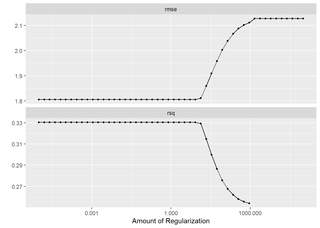
Yes, it visualizes how the performance metrics are impacted by our parameter choice of the regularization parameter, i.e, penalty \(\lambda\).
We can also collect the metrics:
# A tibble: 100 × 7
penalty .metric .estimator mean n std_err .config
<dbl> <chr> <chr> <dbl> <int> <dbl> <chr>
1 0.00001 rmse standard 1.81 2 0.0361 Preprocessor1_Model01
2 0.00001 rsq standard 0.330 2 0.0530 Preprocessor1_Model01
3 0.0000160 rmse standard 1.81 2 0.0361 Preprocessor1_Model02
4 0.0000160 rsq standard 0.330 2 0.0530 Preprocessor1_Model02
5 0.0000256 rmse standard 1.81 2 0.0361 Preprocessor1_Model03
6 0.0000256 rsq standard 0.330 2 0.0530 Preprocessor1_Model03
7 0.0000409 rmse standard 1.81 2 0.0361 Preprocessor1_Model04
8 0.0000409 rsq standard 0.330 2 0.0530 Preprocessor1_Model04
9 0.0000655 rmse standard 1.81 2 0.0361 Preprocessor1_Model05
10 0.0000655 rsq standard 0.330 2 0.0530 Preprocessor1_Model05
# ℹ 90 more rows
Afterwards select_best() can be used to extract the best parameter value.
# Extract best penalty after tuning
best_penalty <- select_best(tune_result, metric = "rsq")
best_penalty# A tibble: 1 × 2
penalty .config
<dbl> <chr>
1 0.00001 Preprocessor1_Model01Finalize workflow, assess accuracy and extract predicted values
Finally, we can update our workflow with finalize_workflow() and set the penalty to best_penalty that we stored above, and fit the model on our training data.
══ Workflow ════════════════════════════════════════════════════════════════════
Preprocessor: Recipe
Model: linear_reg()
── Preprocessor ────────────────────────────────────────────────────────────────
3 Recipe Steps
• step_dummy()
• step_zv()
• step_normalize()
── Model ───────────────────────────────────────────────────────────────────────
Linear Regression Model Specification (regression)
Main Arguments:
penalty = 0.00001
mixture = 0
Computational engine: glmnet
We then evaluate the accuracy of this model (that is based on the training data) using the test data data_test. We use augment() to obtain the predictions:
# A tibble: 174 × 201
respondent_id life_satisfaction country unemployed_active unemployed
<dbl> <dbl> <fct> <dbl> <dbl>
1 10125 7 FR 0 0
2 10349 9 FR 0 0
3 10358 9 FR 0 0
4 10436 8 FR 0 0
5 10625 7 FR 0 0
6 10663 6 FR 0 0
7 10701 8 FR 0 0
8 10726 6 FR 0 0
9 10742 6 FR 0 0
10 10743 8 FR 0 0
# ℹ 164 more rows
# ℹ 196 more variables: education <dbl>, news_politics_minutes <dbl>,
# internet_use_frequency <ord>, trust_people <dbl>, people_fair <dbl>,
# people_helpful <dbl>, political_interest <ord>, system_allows_say <ord>,
# active_role_politics <ord>, system_allows_influence <ord>,
# confident_participate_politics <ord>, trust_parliament <dbl>,
# trust_legal_system <dbl>, trust_police <dbl>, trust_politicians <dbl>, …And can directly pipe the result into functions such as rsq(), rmse() and mae() to obtain the corresponding measures of accuracy.
# A tibble: 1 × 3
.metric .estimator .estimate
<chr> <chr> <dbl>
1 rsq standard 0.411# A tibble: 1 × 3
.metric .estimator .estimate
<chr> <chr> <dbl>
1 rmse standard 1.72# A tibble: 1 × 3
.metric .estimator .estimate
<chr> <chr> <dbl>
1 mae standard 1.299 Lab: Tuning lasso
# Define the recipe
recipe2 <- recipe(life_satisfaction ~ ., data = data_train) %>%
step_zv(all_numeric_predictors()) %>% # remove predictors with zero variance
step_normalize(all_numeric_predictors()) %>% # normalize predictors
step_dummy(all_nominal_predictors())
# Specify the model
model2 <-
linear_reg(penalty = tune(), mixture = 1) %>%
set_mode("regression") %>%
set_engine("glmnet")
# Define the workflow
workflow2 <- workflow() %>%
add_recipe(recipe2) %>%
add_model(model2)
# Define the penalty grid
penalty_grid <- grid_regular(penalty(range = c(-2, 2)), levels = 50)
# Tune the model and visualize
tune_result <- tune_grid(
workflow2,
resamples = data_folds,
grid = penalty_grid
)
autoplot(tune_result)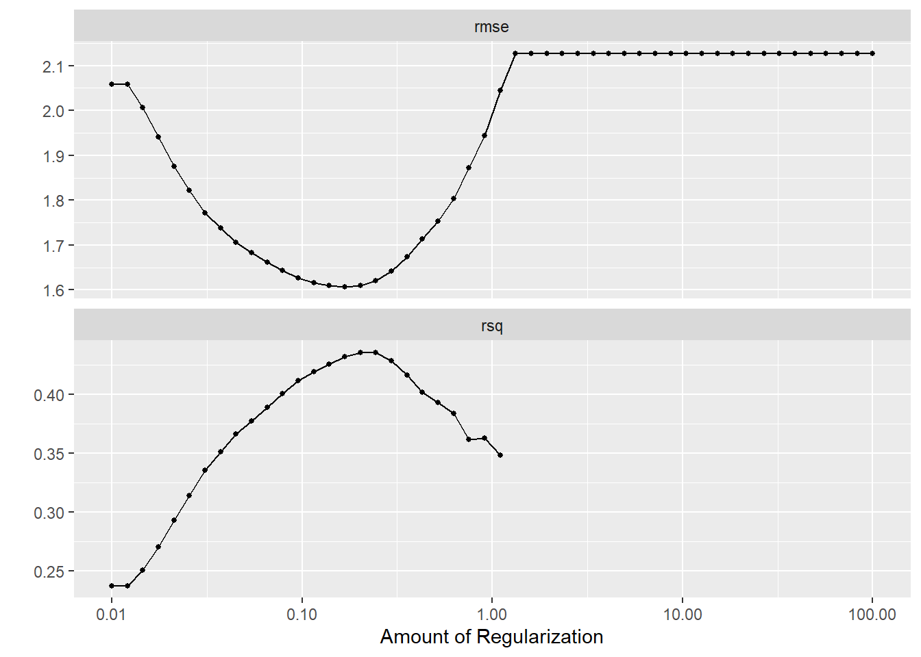
# Select best penalty
best_penalty <- select_best(tune_result, metric = "rsq")
# Finalize workflow and fit model
workflow_final <- finalize_workflow(workflow2, best_penalty)
fit_final <- fit(workflow_final, data = data_train)
# Check accuracy in training data
augment(fit_final, new_data = data_train) %>%
mae(truth = life_satisfaction, estimate = .pred)# A tibble: 1 × 3
.metric .estimator .estimate
<chr> <chr> <dbl>
1 mae standard 1.12# A tibble: 174 × 201
respondent_id life_satisfaction country unemployed_active unemployed
<dbl> <dbl> <fct> <dbl> <dbl>
1 10125 7 FR 0 0
2 10349 9 FR 0 0
3 10358 9 FR 0 0
4 10436 8 FR 0 0
5 10625 7 FR 0 0
6 10663 6 FR 0 0
7 10701 8 FR 0 0
8 10726 6 FR 0 0
9 10742 6 FR 0 0
10 10743 8 FR 0 0
# ℹ 164 more rows
# ℹ 196 more variables: education <dbl>, news_politics_minutes <dbl>,
# internet_use_frequency <ord>, trust_people <dbl>, people_fair <dbl>,
# people_helpful <dbl>, political_interest <ord>, system_allows_say <ord>,
# active_role_politics <ord>, system_allows_influence <ord>,
# confident_participate_politics <ord>, trust_parliament <dbl>,
# trust_legal_system <dbl>, trust_police <dbl>, trust_politicians <dbl>, …# Assess accuracy (RSQ)
augment(fit_final, new_data = data_test) %>%
  rsq(truth = life_satisfaction, estimate = .pred)
# A tibble: 1 × 3
.metric .estimator .estimate
<chr> <chr> <dbl>
1 rsq standard 0.526# Assess accuracy (MAE)
augment(fit_final, new_data = data_test) %>%
    mae(truth = life_satisfaction, estimate = .pred)
# A tibble: 1 × 3
.metric .estimator .estimate
<chr> <chr> <dbl>
1 mae standard 1.0710 Lab: Tuning XGBoost model
Below we use XGBoost to built a predictive model of life satisfaction. See here for another example. And Section 7.2.1 for and example of refining parameters after a first automated grid search.
    set.seed(345)

# Extract data with missing outcome
  data_missing_outcome <- data %>% filter(is.na(life_satisfaction))
  dim(data_missing_outcome)
[1] 205 346# Omit individuals with missing outcome from data
data <- data %>% drop_na(life_satisfaction) # ?drop_na
dim(data)[1] 1772 346# STEP 2
# Split the data into training and test data
data_split <- initial_split(data, prop = 0.80)
data_split # Inspect<Training/Testing/Total>
<1417/355/1772> # Extract the two datasets
data_train <- training(data_split)
data_test <- testing(data_split) # Do not touch until the end!
# Create resampled partitions
data_folds <- vfold_cv(data_train, v = 5) # V-fold/k-fold cross-validation
data_folds # data_folds now contains several resamples of our training data # 5-fold cross-validation
# A tibble: 5 × 2
splits id
<list> <chr>
1 <split [1133/284]> Fold1
2 <split [1133/284]> Fold2
3 <split [1134/283]> Fold3
4 <split [1134/283]> Fold4
5 <split [1134/283]> Fold5 # Define recipe
recipe1 <-
recipe(formula = life_satisfaction ~ ., data = data_train) %>%
update_role(respondent_id, new_role = "ID") %>% # Declare ID variable
step_filter_missing(all_predictors(), threshold = 0.01) %>%
step_naomit(life_satisfaction, all_predictors()) %>% # better deal with missings beforehand
step_nzv(all_predictors(), freq_cut = 0, unique_cut = 0) %>% # remove variables with zero variances
#step_novel(all_nominal_predictors()) %>% # prepares data to handle previously unseen factor levels
step_unknown(all_nominal_predictors()) %>% # categorizes missing categorical data (NA's) as `unknown`
step_dummy(all_nominal_predictors())# %>% # dummy codes categorical variables
#step_zv(all_predictors()) %>% # remove vars with only single value
#step_normalize(all_predictors()) # normale predictors
# Inspect the recipe
recipe1
# Check preprocessed data
data_preprocessed <- prep(recipe1, data_train)$template
dim(data_preprocessed)[1] 1258 212# Specify model with tuning
model1 <-
boost_tree(
trees = 1000,
min_n = tune(), # Tune (see ?details_boost_tree_xgboost)
mtry = tune(),
stop_iter = tune(),
learn_rate = 0.01, # Choose higher value for speed (e.g., 0.3)
loss_reduction = tune(),
sample_size = tune()
) %>%
set_engine("xgboost") %>%
set_mode("regression")
# Specify workflow (with tuning)
workflow1 <- workflow() %>%
add_recipe(recipe1) %>%
add_model(model1)
## Step 4: Tune, evaluate the model using resampling and choose/explore the best model
# Specify to use parallel processing
doParallel::registerDoParallel()
tune_result <- tune_grid(
workflow1,
resamples = data_folds,
metrics = metric_set(mae, rmse, rsq), # Specify which metrics to calculate
grid = 50 # Choose grid points automatically; Pick lower value for speed
)
tune_result# Tuning results
# 5-fold cross-validation
# A tibble: 5 × 4
splits id .metrics .notes
<list> <chr> <list> <list>
1 <split [1133/284]> Fold1 <tibble [150 × 9]> <tibble [0 × 3]>
2 <split [1133/284]> Fold2 <tibble [150 × 9]> <tibble [0 × 3]>
3 <split [1134/283]> Fold3 <tibble [150 × 9]> <tibble [0 × 3]>
4 <split [1134/283]> Fold4 <tibble [150 × 9]> <tibble [0 × 3]>
5 <split [1134/283]> Fold5 <tibble [150 × 9]> <tibble [0 × 3]># A tibble: 150 × 11
mtry min_n loss_reduction sample_size stop_iter .metric .estimator mean
<int> <int> <dbl> <dbl> <int> <chr> <chr> <dbl>
1 182 8 0.00000213 0.478 18 mae standard 1.18
2 182 8 0.00000213 0.478 18 rmse standard 1.63
3 182 8 0.00000213 0.478 18 rsq standard 0.475
4 161 12 0.300 0.237 5 mae standard 1.19
5 161 12 0.300 0.237 5 rmse standard 1.63
6 161 12 0.300 0.237 5 rsq standard 0.473
7 193 19 0.0546 0.144 4 mae standard 1.21
8 193 19 0.0546 0.144 4 rmse standard 1.64
9 193 19 0.0546 0.144 4 rsq standard 0.466
10 91 32 18.1 0.285 14 mae standard 1.19
# ℹ 140 more rows
# ℹ 3 more variables: n <int>, std_err <dbl>, .config <chr># Visualize accuracy for different hyperparameters
tune_result %>%
collect_metrics() %>% # extract metrics
filter(.metric == "mae") %>% # keep mae only
select(mean, mtry:stop_iter) %>% # subset variables
pivot_longer(mtry:stop_iter, # convert to longer
values_to = "value",
names_to = "parameter"
) %>%
ggplot(aes(value, mean, color = parameter)) + # plot!
geom_point(show.legend = FALSE) +
facet_wrap(~parameter, scales = "free_x") +
labs(x = NULL, y = "MAE")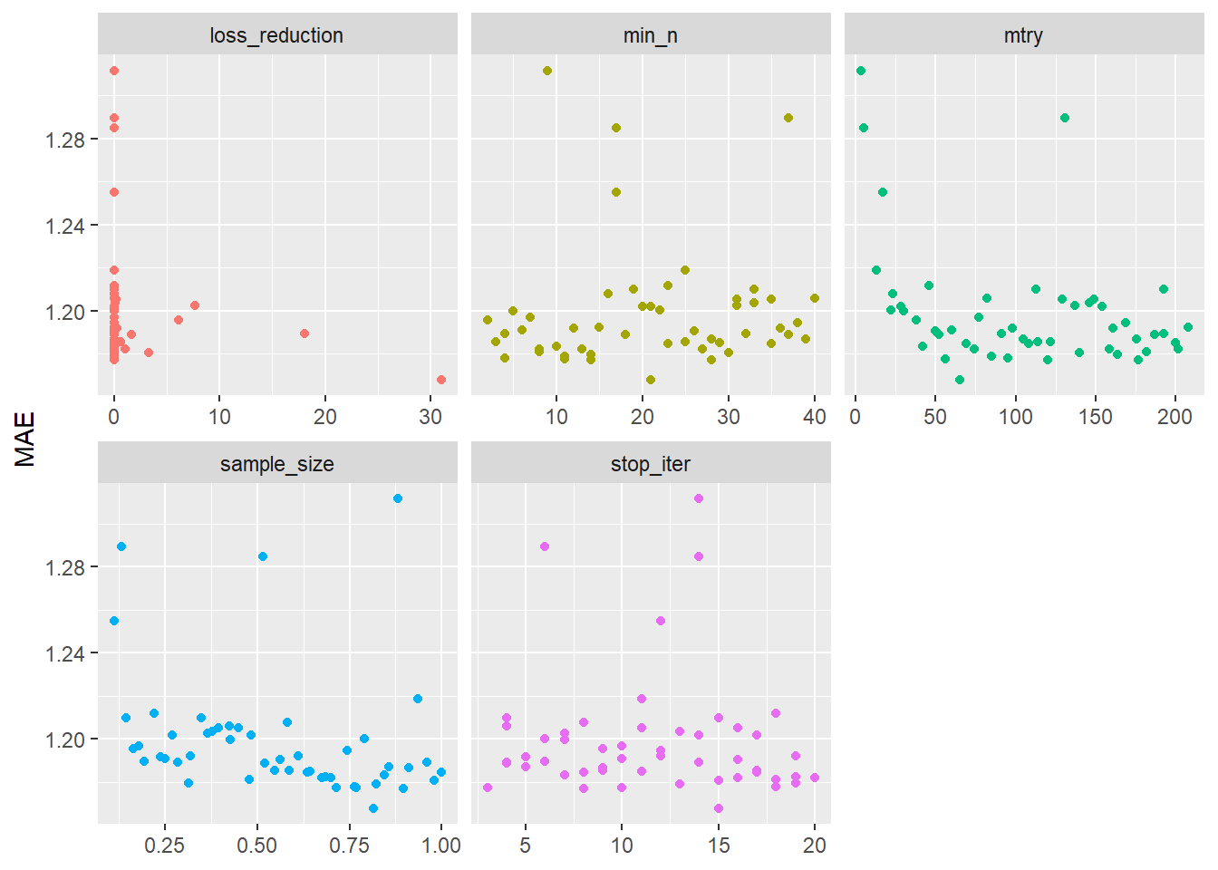
## Choose best model after tuning (for final fit)


# Find tuning parameter combination with best performance values
  best_hyperparameters <- select_best(tune_result, "mae")
  best_hyperparameters
# A tibble: 1 × 6
mtry min_n loss_reduction sample_size stop_iter .config
<int> <int> <dbl> <dbl> <int> <chr>
1 65 21 31.0 0.815 15 Preprocessor1_Model19# Take list/tibble of tuning parameter values
# and update model1 with those values.
model_final <- finalize_model(model1,
parameters = best_hyperparameters # define
)
## Step 5: Fit final model to training data and assess accuracy
# Define final workflow
workflow_final <- workflow() %>%
add_recipe(recipe1) %>% # use standard recipe
add_model(model_final) # use final model
# Fit final model
fit_final <- fit(workflow_final, data = data_train)
fit_final══ Workflow [trained] ══════════════════════════════════════════════════════════
Preprocessor: Recipe
Model: boost_tree()
── Preprocessor ────────────────────────────────────────────────────────────────
5 Recipe Steps
• step_filter_missing()
• step_naomit()
• step_nzv()
• step_unknown()
• step_dummy()
── Model ───────────────────────────────────────────────────────────────────────
##### xgb.Booster
raw: 1.5 Mb
call:
xgboost::xgb.train(params = list(eta = 0.01, max_depth = 6, gamma = 31.0078345415526,
colsample_bytree = 1, colsample_bynode = 0.30952380952381,
min_child_weight = 21L, subsample = 0.814818637915887), data = x$data,
nrounds = 1000, watchlist = x$watchlist, verbose = 0, early_stopping_rounds = 15L,
nthread = 1, objective = "reg:squarederror")
params (as set within xgb.train):
eta = "0.01", max_depth = "6", gamma = "31.0078345415526", colsample_bytree = "1", colsample_bynode = "0.30952380952381", min_child_weight = "21", subsample = "0.814818637915887", nthread = "1", objective = "reg:squarederror", validate_parameters = "TRUE"
xgb.attributes:
best_iteration, best_msg, best_ntreelimit, best_score, niter
callbacks:
cb.evaluation.log()
cb.early.stop(stopping_rounds = early_stopping_rounds, maximize = maximize,
verbose = verbose)
# of features: 210
niter: 784
best_iteration : 769
best_ntreelimit : 769
best_score : 1.396942
best_msg : [769] training-rmse:1.396942
nfeatures : 210
evaluation_log:
iter training_rmse
1 6.871760
2 6.807678
---
783 1.396945
784 1.396945# Q: What do the values for `mtry` and `min_n` in the final model mean?
# Check accuracy in for full training data
metrics_combined <- metric_set(rsq, rmse, mae) # Set accuracy metrics
augment(fit_final, new_data = data_train) %>%
metrics_combined(truth = life_satisfaction, estimate = .pred) # A tibble: 3 × 3
.metric .estimator .estimate
<chr> <chr> <dbl>
1 rsq standard 0.587
2 rmse standard 1.47
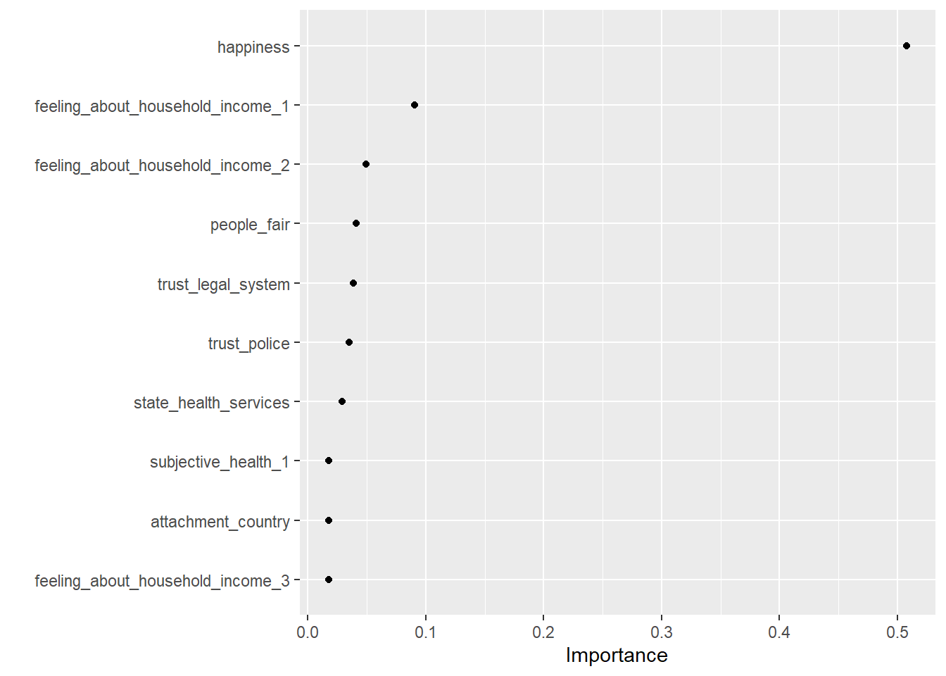
3 mae standard 1.07 # Visualize variable importance
# install.packages("vip")
library(vip)
fit_final$fit$fit %>%
vip::vi() %>%
kable()| Variable | Importance |
|---|---|
| happiness | 0.5076624 |
| feeling_about_household_income_1 | 0.0906490 |
| feeling_about_household_income_2 | 0.0492847 |
| people_fair | 0.0409148 |
| trust_legal_system | 0.0384230 |
| trust_police | 0.0350243 |
| state_health_services | 0.0289000 |
| subjective_health_1 | 0.0179967 |
| attachment_country | 0.0176359 |
| feeling_about_household_income_3 | 0.0175809 |
| feeling_about_household_income_4 | 0.0129863 |
| people_helpful | 0.0078076 |
| trust_people | 0.0066881 |
| internet_use_frequency_1 | 0.0054451 |
| religiousness | 0.0051567 |
| age | 0.0051280 |
| education | 0.0050878 |
| news_politics_minutes | 0.0046871 |
| value_trying_new_things_5 | 0.0046060 |
| year_of_birth | 0.0045159 |
| religious_service_attendance_7 | 0.0041422 |
| social_meetings_3 | 0.0037735 |
| subjective_health_5 | 0.0035604 |
| social_meetings_1 | 0.0030801 |
| maritalb_5 | 0.0029037 |
| respondent_overall_experience | 0.0028811 |
| domicile_description_5 | 0.0026771 |
| value_fun_pleasure_2 | 0.0025720 |
| domicile_description_3 | 0.0025445 |
| religious_service_attendance_1 | 0.0024494 |
| children_learns_obedience_3 | 0.0024386 |
| communication_feels_closer | 0.0024155 |
| social_activities_1 | 0.0023406 |
| internet_use_frequency_3 | 0.0022830 |
| value_fun_pleasure_1 | 0.0022033 |
| discrimination_group_membership | 0.0020472 |
| religious_service_attendance_5 | 0.0019954 |
| climate_change_personal_responsibility | 0.0019159 |
| social_activities_2 | 0.0017640 |
| religious_service_attendance_4 | 0.0017352 |
| value_security_1 | 0.0013886 |
| social_activities_4 | 0.0013504 |
| maritalb_2 | 0.0012951 |
| discrimination_not_applicable | 0.0012828 |
| political_interest_2 | 0.0012350 |
| daily_activities_hampered_1 | 0.0012105 |
| value_trying_new_things_4 | 0.0011043 |
| social_meetings_2 | 0.0010342 |
| maritalb_6 | 0.0010013 |
| domicile_description_1 | 0.0009721 |
| value_loyalty_to_friends_4 | 0.0009333 |
| value_wealth_1 | 0.0008996 |
| value_fun_pleasure_3 | 0.0008383 |
| value_trying_new_things_2 | 0.0008354 |
| social_meetings_6 | 0.0008211 |
| value_wealth_5 | 0.0008061 |
| political_interest_1 | 0.0007280 |
| climate_change_worry_3 | 0.0007119 |
| household_members | 0.0007017 |
| value_trying_new_things_6 | 0.0006768 |
| political_interest_4 | 0.0006616 |
| value_trying_new_things_3 | 0.0006517 |
| female | 0.0006365 |
| religious_service_attendance_6 | 0.0006057 |
| political_interest_3 | 0.0006047 |
| social_meetings_7 | 0.0005771 |
| daily_activities_hampered_3 | 0.0005714 |
| value_security_3 | 0.0005685 |
| internet_use_frequency_2 | 0.0005517 |
| parents_alive_1 | 0.0005433 |
| value_wealth_2 | 0.0005127 |
| value_trying_new_things_1 | 0.0004846 |
| value_security_2 | 0.0004772 |
| value_loyalty_to_friends_5 | 0.0004741 |
| value_equality_4 | 0.0004700 |
| social_activities_5 | 0.0004681 |
| climate_change_administration_1 | 0.0004538 |
| value_fun_pleasure_4 | 0.0004510 |
| internet_use_frequency_5 | 0.0004376 |
| climate_change_cause_5 | 0.0004324 |
| discuss_intimate_matters_7 | 0.0004312 |
| children_over_12_number | 0.0004052 |
| maritalb_1 | 0.0003836 |
| subjective_health_4 | 0.0003603 |
| courts_equal_treatment | 0.0003555 |
| value_understanding_others_5 | 0.0003546 |
| social_meetings_5 | 0.0003519 |
| discuss_intimate_matters_6 | 0.0003441 |
| value_understanding_others_4 | 0.0003413 |
| subjective_health_3 | 0.0003357 |
| born_in_country | 0.0003317 |
| internet_access_other | 0.0003233 |
| value_understanding_others_6 | 0.0002969 |
| mnactic_8 | 0.0002956 |
| value_security_5 | 0.0002941 |
| children_learns_obedience_1 | 0.0002932 |
| religious_service_attendance_2 | 0.0002873 |
| mnactic_1 | 0.0002791 |
| value_fun_pleasure_6 | 0.0002783 |
| parents_alive_3 | 0.0002757 |
| value_understanding_others_3 | 0.0002743 |
| value_equality_1 | 0.0002713 |
| discuss_intimate_matters_2 | 0.0002585 |
| value_wealth_4 | 0.0002539 |
| social_activities_3 | 0.0002505 |
| mnactic_2 | 0.0002500 |
| doing7days_retired | 0.0002438 |
| value_fun_pleasure_5 | 0.0002420 |
| value_understanding_others_1 | 0.0002345 |
| domicile_description_2 | 0.0002333 |
| trade_union_membership_1 | 0.0002318 |
| maritalb_4 | 0.0002280 |
| internet_access_home | 0.0002222 |
| discuss_intimate_matters_1 | 0.0002181 |
| value_equality_5 | 0.0002075 |
| partner_paid_work_last_week | 0.0001657 |
| maritalb_3 | 0.0001256 |
| public_demonstration | 0.0001190 |
| campaign_badge | 0.0001164 |
| discuss_intimate_matters_3 | 0.0001031 |
| mnactic_3 | 0.0001029 |
| mother_born_in_country | 0.0001011 |
| contacted_politician | 0.0000952 |
| ever_divorced | 0.0000944 |
| discuss_intimate_matters_5 | 0.0000943 |
| value_loyalty_to_friends_6 | 0.0000885 |
| religious_service_attendance_3 | 0.0000668 |
| subjective_health_2 | 0.0000631 |
| government_protection_against_poverty | 0.0000630 |
## Step 6: Fit final model to test data and assess accuracy
  augment(fit_final, new_data = data_test) %>%
      metrics_combined(truth = life_satisfaction, estimate = .pred)
# A tibble: 3 × 3
.metric .estimator .estimate
<chr> <chr> <dbl>
1 rsq standard 0.452
2 rmse standard 1.61
3 mae standard 1.16 References
Arnold, Christian, Luka Biedebach, Andreas Küpfer, and Marcel Neunhoeffer. 2024. “The Role of Hyperparameters in Machine Learning Models and How to Tune Them.” Political Science Research and Methods, February, 1–8.
Footnotes
published between 1 January 2016 and 20 October 2021 in some of the top journals of our discipline—the American Political Science Review (APSR), Political Analysis (PA), and Political Science Research and Methods (PSRM)↩︎
The
penaltyparameter refers to the amount of regularization applied to the model. Regularization is a technique used to prevent overfitting by adding apenaltyterm to the loss function, which discourages overly complex models. It helps in improving the model’s ability to generalize to unseen data by reducing the variance in the model’s predictions.
Lasso regression adds apenaltyterm to the loss function equal to the absolute value of the coefficients’ sum multiplied by a regularization parameter (lambdaoralpha). Thepenaltyparameter in tidymodels specifies the strength of this regularization term for Lasso regression. Higher values ofpenaltyresult in more regularization, leading to more coefficients being pushed towards zero, potentially resulting in a sparse model (some coefficients become exactly zero), which aids in feature selection.
Ridge regression, on the other hand, adds apenaltyterm to the loss function equal to the squared sum of the coefficients multiplied by a regularization parameter (lambdaoralpha). Similarly, thepenaltyparameter in tidymodels specifies the strength of this regularization term for Ridge regression. Higher values ofpenaltyresult in stronger regularization, but unlike Lasso, Ridge tends to shrink all coefficients towards zero proportionally without necessarily causing them to become zero, which helps in reducing multicollinearity.↩︎By adjusting the “tree_depth” parameter, you control the complexity of each individual decision tree in the XGBoost ensemble. Higher values allow the tree to capture more complex patterns in the data but may also increase the risk of overfitting. Conversely, lower values restrict the complexity of the tree, potentially improving generalization but may lead to underfitting if set too low.↩︎
treesdetermines the complexity and capacity of the model. More trees can potentially capture more complex patterns in the data but may also lead to overfitting if not controlled properly.↩︎learn_rateparameter, also known as the learning rate or eta in the context of XGBoost, is a crucial hyperparameter that influences the training process of gradient boosting algorithms, including XGBoost. The learning rate determines the step size or the rate at which the model updates its weights or parameters during the training process. It’s a scalar value that controls how much we are adjusting the weights of our network with respect to the loss gradient.↩︎The
loss_reductionparameter plays a role in controlling the construction of individual decision trees during the boosting process. Theloss_reductionparameter specifies the minimum amount of reduction in the loss function required to make a further partition on a leaf node of the decision tree. Essentially, it determines the threshold for splitting a node based on the improvement in the model’s performance.↩︎The
sample_sizeparameter specifies the proportion of observations sampled for each tree during the training process. Gradient boosting algorithms, including XGBoost, often use a technique called “bootstrapping” or “bagging” to train individual trees. In each iteration of training, a random subset of observations is sampled with replacement from the original dataset.↩︎The
stop_iterparameter is related to early stopping during the model training process. Early stopping is a technique used during the training of machine learning models to prevent overfitting and improve efficiency. Instead of training the model for a fixed number of iterations (or epochs), early stopping monitors a performance metric (e.g., validation loss) during training and stops training when the performance metric stops improving.↩︎