| 0 | 1 | 2 | 3 | 4 | 5 | 6 | 7 | 8 | 9 | 10 |
|---|---|---|---|---|---|---|---|---|---|---|
| 34 | 14 | 42 | 49 | 76 | 170 | 169 | 323 | 462 | 212 | 213 |
Introduction
Questions/Learning outcomes:
- How can we define AI/ML?
- How does the AI landscape develop?
- What are the fundamental AI debates?
- How is AI/ML used in the social sciences?
- What is the difference between classical statistics/modelling and machine learning?
- What is the difference between descriptive, causal and predictive inference/research questions?
The material for the following sessions is based on James et al. (2013), Molina and Garip (2019), James et al. (2013), Chollet and Allaire (2018) and others’ work (including some of my own).
1 Artificial intelligence & machine learning
1.1 What is AI?

“Artificial intelligence (AI) is intelligence - perceiving, synthesizing, and inferring information - demonstrated by machines, as opposed to intelligence displayed by non-human animals and humans. Example tasks in which this is done include speech recognition, computer vision, translation between (natural) languages, as well as other mappings of inputs.” (Wikipedia)
- “the effort to automate intellectual tasks normally performed humans” (Chollet and Allaire 2018, 2) (includes chess computers!)
1.2 Definitions: What is machine learning?
“Machine learning (ML) is a field of inquiry devoted to understanding and building methods that ”learn” […] It is seen as a part of artificial intelligence.” (Wikipedia)
- “Machine learning is programming computers to optimize a performance criterion using example data or past experience.” (Alpaydin 2014, 3)
- “Machine learning is a specific subfield of AI that aims at automatically developing programs (called models) purely from exposure to training data. This process of turning models data into a program is called learning.” (Chollet and Allaire 2018, 307)
Data mining: “Application of machine learning methods to large databases is called data mining. The analogy is that a large volume of earth and raw material is extracted from a mine, which when processed leads to a small amount of very precious material; similarly, in data mining, a large volume of data is processed to construct a simple model with valuable use, for example, having high predictive accuracy.” (Alpaydin 2014, 2)
1.3 The AI landscape
- Different Actors with varying interests: Q: What are the aims/interests of different actors below?
- Researchers (public institutions), e.g., LeCun, Hinton, Bengio (Turing Award: Nobel Prize of computing)
- Companies: Google (Deepmind), Facebook, Microsoft (OpenAI), Baidu, etc. (Zand, Scheuermann, and Spiegel 2018)
- Countries
- Individuals
- History (Domingos 2015; Buchanan 2005; Roser 2022): Skepticism warranted.. who writes the history?
- Chollet and Allaire (2018, 2f)
- 1950s (“can we make computers ‘think’”)
- Symbolic AI: Dominant paradigm from 1950s to 1980s (peak popularity)
- Idea: handcraft sufficiently large set of explicit rules for manipulating knowledge
- Works for well-defined, logical problems such as chess but not for complex, fuzzy problems (image classification, speech recognition)
- Idea: handcraft sufficiently large set of explicit rules for manipulating knowledge
- Machine learning: Took off in the 1990s
- Chollet and Allaire (2018, 2f)
Insights
- Various actors with varying interests that can often be subsumed under the concept of “competition”. In their daily lives individuals would simply like AI to just work (but are often not aware that AI is working in the background).
- There are various books that summarize the history of AI. Importantly, theses surveys may be biased towards certain people/contexts.
1.4 Stats on the field of AI
1.4.1 Investments, ability, costs, affiliation
- See Our World in Data for various graphs
- Ability: Chess ability of the best computers
- Costs: Cost to train an AI system to equivalent performance on ImageNet
- Computation used to train notable artificial intelligence systems (FLOPS)
- Affiliation of research teams
- Affiliation of researchers behind notable AI systems
- Number of datapoints used to train notable artificial intelligence systems
- Share of women among new artificial intelligence and computer science PhDs in the US and Canada
Insights
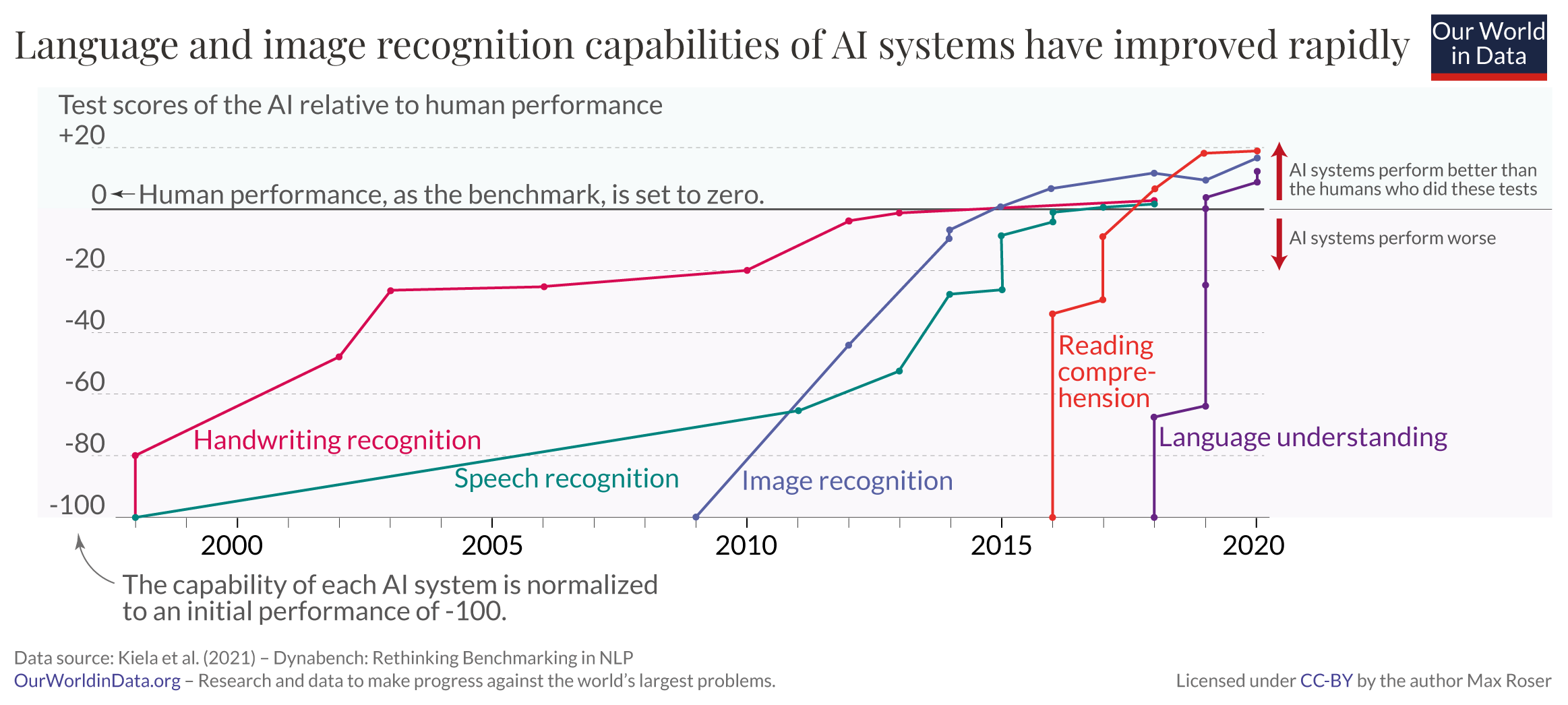
- Massive investments in the last years
- Ability: Best chess players are now beaten by ML algorithms.. a few years ago already actually (same for GO!)
- Costs: Costs go down over time but… (Imagenet)
- …computation underlying training of recently successful models is extremely high -> super computers (for notable DL systems!)
- Research as moved into industry away from universities
- Size of datasets necessary to train has grown for notable DL systems!
- Share of women in AI/Computer science is low.. (possible bias!)
- See, e.g., Our World in Data, Statista and OECD.ai for more statistics
- AI timelines: What do experts in artificial intelligence expect for the future?
1.4.2 Language and image recognition capabilities
2 Debates around AI/ML
- There are various larger interlinked debates in the field
- [How well] Does AI really work?
- “Rebooting AI” (Marcus and Davis 2019), etc.
- How should AI be tested? (e.g., competitions etc.)
- Interpretable machine learning (e.g. Molnar 2022)
- Bias of ML algorithms (training data, personnel, minorities) (e.g., Metz 2022, Ch. 15)
- “I call it a sea of dudes”1
- Garbage in, garbage out; reproduction of inequalities (rental/loan markets)
- Weaponization (e.g., Metz 2022, Ch. 16)
- General adversarial networks (GANS) + adversarial attacks (e.g., Metz 2022, Ch. 13, 212)
- Book: “Weapons of Math Destruction” by Cathy O’Neill
- Artificial general intelligence, Technological singularity, Super intelligence
2.1 Interpretable machine learning
3 Machine learning tasks in the social sciences
- Within social sciences ML is used for various tasks as summarized by Grimmer, Roberts, and Stewart (2021)
- We’ll focus on prediction! (beware of ambiguity of “prediction”)

4 Classical statistics vs. machine learning (skipped)
Questions/Learning outcomes: Understand difference between classic statistics and machine learning.
4.1 Cultures and goals
- Two cultures of statistical analysis (Breiman 2001; Molina and Garip 2019, 29)
- Data modeling vs. algorithmic modeling (Breiman 2001)
- \(\approx\) generative modelling vs. algorithmic modeling (Donoho 2017)
- Data modeling vs. algorithmic modeling (Breiman 2001)
- Generative modeling (classical statistics, Objective: Inference/explanation)
- Goal: understand how an outcome is related to inputs
- Analyst proposes a stochastic model that could have generated the data, and estimates the parameters of the model from the data
- Leads to simple and interpretable models BUT often ignores model uncertainty and out-of-sample performance
- Predictive modeling (Objective: Prediction)
- Goal: prediction, i.e., forecast the outcome for unseen (Q: ?) or future observations
- Analyst treats underlying generative model for data as unknown and primarily considers the predictive accuracy of alternative models on new data
- Leads to complex models that perform well out of sample BUT can produce black-box results that offer little insight on the mechanism linking the inputs to the output (but Interpretable ML)
- Example: Predicting/explaining unemployment with a linear regression model
- See also James et al. (2013, Ch. 2.1.1)
4.2 Machine learning as programming (!) paradigm
- ML reflects a different programming paradigm (Chollet and Allaire 2018, chap. 1.1.2)
- Machine learning arises from this question: could a computer […] learn on its own how to perform a specified task? […] Rather than programmers crafting data-processing rules by hand, could a computer automatically learn these rules by looking at data?
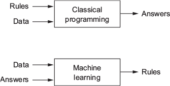
- Classical programming (paradigm of symbolic AI)
- Humans input rules (a program) and data to be processed according to these rules, and out come answers
- Machine learning paradigm
- Humans input data + answers expected from the data, and out come the rules [these rules can then be applied to new data]
- ML system is trained rather than explicitly programmed
- Trained: Presented with many examples relevant to a task → finds statistical structure in these examples &rarr allows system to come up with rules for automating the task (remember Alpha Go)
- Role of math
- While related to math. statistics, ML tends to deal with large, complex datasets (e.g., millions of images, each consisting of thousands of pixels)
- As a result ML (especially deep learning) exhibits comparatively little mathematical theory and is engineering oriented (ideas proven more often empirically than mathematically) (Chollet and Allaire 2018, chap. 1.1.2)
5 Terminology
5.1 Terminological differences (1)
Terminology is a source of confusion (Athey and Imbens 2019, 689)
Q: Do you know any machine learning terminology?
Statistical learning vs. machine learning (ML) (James et al. 2013, 1)
- Terms reflect disciplinary origin (statistics vs. computer science)
- We will use the two as synonyms (as well as AI)
Regression problem: Prediction of a continuous or quantitative output values (James et al. 2013, 2)
- e.g., predict wage using age, education and year
Classification problem: Prediction of a non-numerical value—that is, a categorical or qualitative output
- e.g., predict increase/decrease of stock market on a given day using previous movements
Q: What does the “inference” in statistical inference stand for? (Population vs. sample)
5.2 Terminological differences (2)
- Terminology: Well-established older labels vs. “new” terminology
- Sample used to estimate the parameters vs. training sample
- Model is estimated vs. Model is trained/fitted
- Regressors, covariates, predictors vs. features (or inputs)
- Dependent variable/outcome vs. output
- Regression parameters (coefficients) vs. weights
5.3 Supervised vs. unsupervised learning
- Supervised vs. unsupervised machine learning (James et al. 2013, 1; Athey and Imbens 2019, 689)
- Unsupervised statistical learning: There are inputs but no supervising output; we can still learn about relationships and structure from such data
- Only observe \(X_{i}\) and try to group them into clusters
- Supervised statistical learning: involves building a statistical model for predicting, or estimating, an output based on one or more inputs
- We observe both features \(x_{i}\) and the outcome \(y_{i}\)
- Use the model to predict unobserved outcomes \((y_{i})\) of units \(i\) where we only have \(x_{i}\)
- Unsupervised statistical learning: There are inputs but no supervising output; we can still learn about relationships and structure from such data
- Good analogy: Child in Kindergarden sorts toys (with or without teacher’s input)
6 Data & dimensionality
Questions/Learning outcomes: * Quick repetition of what data/dimensions is/are.
6.1 Data: (Empirical) Univariate distributions
| 0 | 1 |
|---|---|
| 1737 | 27 |
| 0 | 1 | 2 | 3 | 4 | 5 | 6 |
|---|---|---|---|---|---|---|
| 172 | 156 | 411 | 354 | 242 | 132 | 297 |
- Q: Where are most individuals located on the life_satisfaction and unemployed scales?
- Q: Why is data sparsity general a problem?
6.2 Data: (Empirical) Joint distributions
- Measurement process: Assign individuals to cells → distribute across cells → distribution
- 1 variable → univariate distribution
- 2+ variables → multivariate joint distribution
- Q: Above units are grouped on three variables (= dimensions): Life Satisfaction (Y) [0-10], Unemployed (D) [0,1] and Education (X) [0-6]
- How many cells? How many dimensions? (How about time?) Jitter?
- What would the corresponding dataset/dataframe look like?
- What would a joint distribution with 4 variables look like? Can we visualize it?
- What is a conditional distribution?
- What if two variables are perfectly correlated? What does the joinz distribution look like?
- What is the curse of dimensionality?
Insights
- Number of cells/dimensions: \(11*2*7 = 154\) cells; \(3\) dimensions (= variables)
- Corresponding dataset/dataframe: 3 columns * n rows
- Joint distribution with 4 variables
- Hard to imagine.. but if the 4th dimension is categorical then one could generate several 3-dimensional plots
- Conditional distribution: e.g., joint distribution of life satisfaction and unemployed conditional on education = 2 (a slice)
- Perfect correlation: All data points on one line/plane
- Curse of dimensionality: refers to various challenges and limitations that arise when working with high-dimensional data in machine learning and other fields
- As number of features or dimensions in dataset increases, several problems emerge, making it increasingly difficult to analyze and model the data effectively
- Sparsity of Data: In high-dimensional spaces, data points tend to become increasingly sparse. As the number of dimensions grows, the volume of the space increases exponentially, and the available data becomes more thinly spread out. This sparsity can lead to difficulties in estimating densities, making it harder to identify meaningful patterns within the data.
- ..also increased computational complexity, higher danger of overfitting and increased data requirements (ideally enough data to cover space)
6.3 Data: One more joint distribution
Insights
- Always consider how much data you have in certain regions of your outcome variable and features/predictors.
- Big difference between what variable values (and value combinations) we may theoretically vs. empirically observe.
6.4 Data: Probability Distributions (skipped)
- Sometimes called theoretical distributions (as opposed to empirical)
- Invented by mathematicians/statisticians
- Q: What is the most famous one? Who invented it? Others?
- Discrete and continuous probability distributions
- Uni- and multivariate probability distributions
- e.g. multivariate normal: What is the 3rd dimension?
- Q: Facilitate our work… why? What assumptions can we make?
- When we draw from a probability distribution we also simply generate (artificial) data
- R:
rbinom(10, 1, 0.2)= 0, 0, 0, 0, 0, 0, 0, 0, 1, 0
- R:
6.5 Data: Probability Distributions & Inference (skip!)
- We need probability distributions for stat. inference (learning from sample about the population)
- Frequentism/Frequentist inference
- Any given experiment (dataset) can be considered as one of an infinite sequence of possible repetitions of the same experiment (datasets)
- Sample of students in class = one of infinite sequences of sample we could draw from Mannheim Univ. students
- Sample → Calculate mean/regression coefficient → Sampling distribution of statistic \(\approx\) probability distribution
- Bayesian inference
6.6 Data: Exercise
- What is the difference between a univariate distribution and a joint distribution? Give examples for both.
- (skipped) What is the difference between an empirical distribution and a theoretical (probability) distribution? Give examples for both.
- We discussed that any variable has a set of theoretically possible values which it can take on. Empirical observations may then be assigned to those values or not. The same is true for value combinations of two or more variables. This all sounds quite abstract.
- Thinking of two variables education (0-4) and life satisfaction (0-10).
- What theoretical values does education have? And life satisfaction?
- When we combine the theoretical values of the two variables, how many combinations are there?
- Imagine you collect empirical data to which values/cells of life satisfaction do you think most observations we be assigned?
- Thinking of two variables education (0-4) and life satisfaction (0-10).
6.7 Models: What is a model?
- Q: In how far is a map a model of the reality?
- Q: In how far is the mean of age a model of age? Thinkking about the people in this workshop.
- Behind any model there is a (joint) distribution
- Model summarizes (joint) distribution with fewer parameters
- e.g. a mean; or intercept/coefficents in linear model
- Statistical Model (SM) (Wikipedia):
- Class of a mathematical model (MM)
- Embodies assumptions about generation of sample data from data of a larger population
- Assumptions describe set of probability distributions
- e.g. sampling distribution of reg. coefficent = normally or t-distributed
- Inherent probability distributions distinguish SMs from MMs (but see also Nonparametric statistics)
7 Research questions & types of inferences
Questions/Learning outcomes:
- What is the difference between normative (vs. empirical analytical), descriptive, causal and predictive research questions?
- What is the difference between descriptive/causal/predictive inference?
- Clarification of different terminology: Inference; Prediction; Forecasting; Imputation; etc.
7.1 Types of RQs
- Normative vs. empirical analytical (positive)
- Should men and women be paid equally? Are men and women paid equally (and why?)?
- What? vs. Why? (Gerring 2012, 722-723)
- What? Describe aspect of the world
- Why? concern causal arguments that hold that one or more phenomena generate change in some outcome (imply a counterfactual)
- My personal preference: descriptive vs. causal vs. predictive questions
7.2 Descriptive research questions
Measure:‘All things considered, how satisfied are you with your life as a whole nowadays? Please answer using this card, where 0 means extremely dissatisfied and 10 means extremely satisfied.’
Descriptive questions (univariate)
- What is Laura’s level of life satisfaction?
- What is the distribution of life satisfaction (Y)?
| 0 | 1 | 2 | 3 | 4 | 5 | 6 | 7 | 8 | 9 | 10 |
|---|---|---|---|---|---|---|---|---|---|---|
| 34 | 14 | 43 | 50 | 76 | 170 | 170 | 324 | 465 | 213 | 213 |
- We can add as many variables/dimensions as we like → multivariate (e.g. gender, time)
- Q: What would the table above look like when we add gender as a second dimension?
- Descriptive questions (multivariate)
- Do females have higher life satisfaction than males?
- Did life satisfaction rise across time?
7.3 Causal research questions (Why?)
| 0 | 1 | 2 | 3 | 4 | 5 | 6 | 7 | 8 | 9 | 10 | |
|---|---|---|---|---|---|---|---|---|---|---|---|
| not unemployed | 31 | 14 | 41 | 50 | 75 | 163 | 166 | 322 | 461 | 213 | 209 |
| unemployed | 3 | 0 | 2 | 0 | 1 | 7 | 4 | 2 | 4 | 0 | 4 |
- Mean employed: 7.05; Mean unemployed: 5.67
- Descriptive questions: Do unemployed have a different/lower level of life satisfaction from/than non-victims?
- Causal questions: Is there a causal effect of unemployment on life satisfaction?
- Insights
- Data underlying descriptive & causal questions is the same
- Causal questions aways concern one (or more) explanatory causal factors
7.4 Predictive research questions
- Examples
- Can we predict recidvidsm (reoffending) of prisoners?
- Can we predict life satisfaction using unemployment?
- How well can we predict recidivism/life satisfaction? (accuracy)
- Abstract
- Can we predict outputs (given our inputs)?
- Is the available data sufficiently informative to learn the relationships between inputs and ouputs?
- Predictions can be made for individuals or groups (averages)
- e.g., Predict Paul’s age or participants’ average age
- Predictions often made for unseen (sometimes future) observations
- Quick summery…and more on that later!
Insights
- Descriptive, causal and predictive questions differ but are all answered based on data
7.5 Inference (1): Descriptive inference
- Goal of descriptive inference: Estimate a parameter in a population (or only sample)
- e.g., Research question: What is the average of life satisfaction/unemployment among French citizens?
| \(\text{Unit i} \quad\) | \(Name \quad\) | \(X1_{i}^{Age} \quad\) | \(X2_{i}^{Educ.} \quad\) | \(Y_{i}^{Lifesat.} \quad\) |
|---|---|---|---|---|
| 1 | Sofia | 29 | 1 | 3 |
| 2 | Sara | 30 | 2 | 2 |
| 3 | José | 28 | 0 | 5 |
| 4 | Yiwei | 27 | 2 | ? |
| 5 | Julia | 25 | 0 | 6 |
| 6 | Hans | 23 | 0 | ? |
| .. | .. | .. | .. | .. |
| 1000 | Hugo | 23 | 1 | 8 |
- Table 1 displays our sample
- Assuming it were the population we could add a vector \(R_{i}\) that indicates whether someone in the population has been sampled (cf. Abadie et al. 2020)
7.6 Inference (2): Causal inference (skipped)
- Goal of causal inference: Identify whether particular cause/treatment \(D\) has a causal effect on \(Y\) in a population
- e.g., Research question: What is the causal effect of unemployment \(D\) on life satisfaction \(Y\) among French citizens?
| \(\text{Unit i} \quad\) | \(Name \quad\) | \(X1_{i}^{Age} \quad\) | \(X2_{i}^{Educ.} \quad\) | \(D_{i}^{Unempl.} \quad\) | \(Y_{i}^{Lifesat.} \quad\) | \(Y_{i}({\color{blue}{0}})\quad\) | \(Y_{i}({\color{red}{1}})\quad\) |
|---|---|---|---|---|---|---|---|
| 1 | Sofia | 29 | 1 | \({\color{red}{1}}\) | 3 | ? | 3 |
| 2 | Sara | 30 | 2 | \({\color{red}{1}}\) | 2 | ? | 2 |
| 3 | José | 28 | 0 | \({\color{blue}{0}}\) | 5 | 5 | ? |
| 4 | Yiwei | 27 | 2 | \({\color{red}{1}}\) | ? | ? | ? |
| 5 | Julia | 25 | 0 | \({\color{blue}{0}}\) | 6 | 6 | ? |
| 6 | Hans | 23 | 0 | \({\color{red}{1}}\) | ? | ? | ? |
| .. | .. | .. | .. | .. | .. | .. | .. |
| 1000 | Hugo | 23 | 1 | \({\color{blue}{0}}\) | 8 | 8 | ? |
7.7 Inference (3): Causal inference (skipped)
Causal inference: Every-day notion of causality \(\rightarrow\) formalized through potential outcomes framework (Rubin 1974, ~2012)
- \(\delta_{i} =\) \(Y_{i}({\color{red}{1}}) - Y_{i}({\color{blue}{0}})\), e.g., \(\delta_{Sofia}\) \(= \text{Life satisfaction}_{Sofia}({\color{red}{Unemployed}}) - \text{Life satisfaction}_{Sofia}({\color{blue}{Employed}})\)
- FPCI (Holland 1986): Either observe \(Y_{i}({\color{red}{1}})\) or \(Y_{i}({\color{blue}{0}})\) … missing data problem!
- Usual focus on average treatment effect: \(ATE = E[Y_{i}(1) - Y_{i}(0)]\) (or ATT)
Designs, methods & models (with examples from my own research)
- experiments (Bauer et al. 2019, Bauer & Clemm 2021, Bauer et al. 2021, Bauer & Poama 2020), matching, instrumental variables (Bauer & Fatke 2014), regression discontinuity design, difference-in-differences, fixed-effects model (Bauer 2015, 2019), etc. (e.g., Gangl 2010 for overview)
Potential outcomes & identification revolution (Imai 2011):
- Statistical inference: Models + statistical assumptions \(\rightarrow\) Causal inference: Models + statistical assumptions + identification assumptions
7.8 Inference (3): Missing data perspective
| \(\text{Unit i} \quad\) | \(Name \quad\) | \(X1_{i}^{Age} \quad\) | \(X2_{i}^{Educ.} \quad\) | \(D_{i}^{Unempl.} \quad\) | \(Y_{i}^{Lifesat.} \quad\) | \(Y_{i}({\color{blue}{0}})\quad\) | \(Y_{i}({\color{red}{1}})\quad\) |
|---|---|---|---|---|---|---|---|
| 1 | Sofia | 29 | 1 | \({\color{red}{1}}\) | 3 | ? | 3 |
| 2 | Sara | 30 | 2 | \({\color{red}{1}}\) | 2 | ? | 2 |
| 3 | José | 28 | 0 | \({\color{blue}{0}}\) | 5 | 5 | ? |
| 4 | Yiwei | 27 | 2 | \({\color{red}{1}}\) | ? | ? | ? |
| 5 | Julia | 25 | 0 | \({\color{blue}{0}}\) | 6 | 6 | ? |
| 6 | Hans | 23 | 0 | \({\color{red}{1}}\) | ? | ? | ? |
| .. | .. | .. | .. | .. | .. | .. | .. |
| 1000 | Hugo | 23 | 1 | \({\color{blue}{0}}\) | 8 | 8 | ? |
- Data perspective: Both causal inference and machine learning are about missing data!
- Causal inference perspective
- Replace (predict) Sofia’s (and others’) missing potential outcome(s) on variable \(\text{Life satisfaction}\) with other people’s observed outcomes!
- Prediction/ML perspective
- Train model to predict missing observations on variable \(\text{Life satisfaction}\) (see “?”s)
7.12 Timeline of statistical learning
- Source: James et al. (2013, 6–7)
- Beginning of the 19th century: Legendre and Gauss - method of least squares
- Earliest form of linear regression (Astronomy)
- 1936: Fisher - Linear Discriminant Analysis
- 1940s: various authors - Logistic Regression
- 1970: Nelder and Wedderburn - Generalized Linear Models (GLM) of which linear and logistic regression are special cases
- By end of the 1970s: Many more techniques available but almost exclusively linear methods
- Fitting non-linear relationships was computationally infeasible at the time
- By the 1980s: Better computing technology facility non-linear methods
- Mid 1980s: Breiman, Friedman, Olshen and Stone - Classification and Regression Trees
- practical implementation including cross-validation for model selection
- 1986: Hastie/Tibshirani coin term “generalized additive models” for a class of non-linear extensions to generalized linear models (+ practical software implementation)
- Since then statistical learning has emerged as a new subfield!
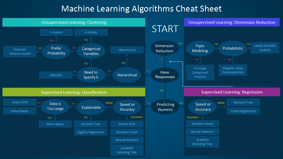
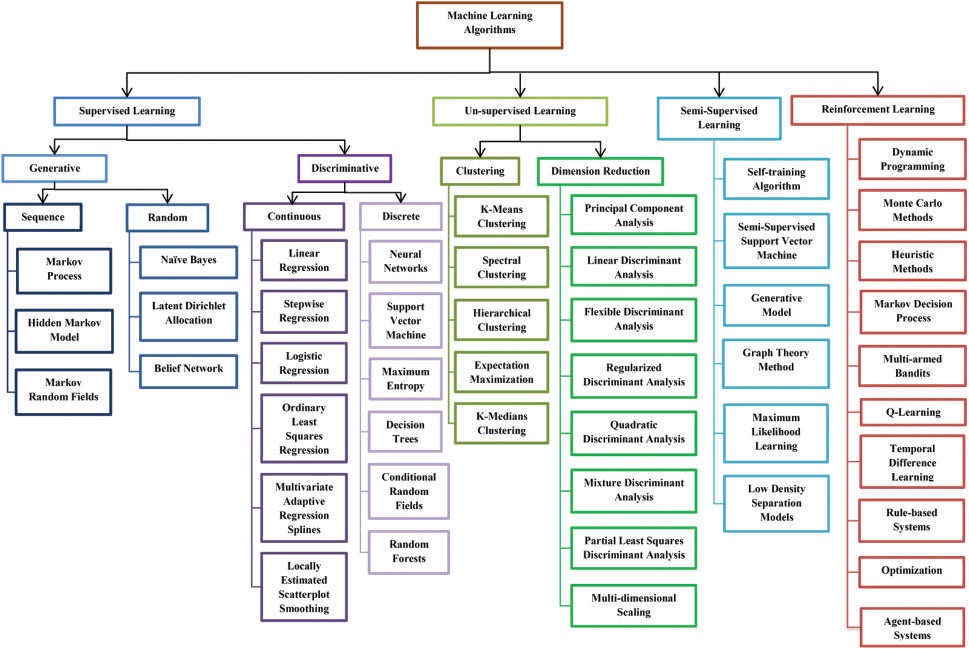
7.13 Machine learning decision tree?
- I tried to find a decision tree outlining different ML methods. Figure 1 seems most helpful (see also Figure 2 and Figure 3).

References
Abadie, Alberto, Susan Athey, Guido W Imbens, and Jeffrey M Wooldridge. 2020. “Sampling-Based Versus Design-Based Uncertainty in Regression Analysis.” Econometrica 88 (1): 265–96.
Alpaydin, Ethem. 2014. Introduction to Machine Learning. MIT Press.
Athey, Susan, and Guido W Imbens. 2019. “Machine Learning Methods That Economists Should Know About.” Annu. Rev. Econom. 11 (1): 685–725.
Breiman, Leo. 2001. “Statistical Modeling: The Two Cultures (with Comments and a Rejoinder by the Author).” SSO Schweiz. Monatsschr. Zahnheilkd. 16 (3): 199–231.
Buchanan, Bruce G. 2005. “A (Very) Brief History of Artificial Intelligence.” AIMag 26 (4): 53–53.
Chollet, Francois, and J J Allaire. 2018. Deep Learning with R. 1st ed. Manning Publications.
Domingos, Pedro. 2015. The Master Algorithm: How the Quest for the Ultimate Learning Machine Will Remake Our World. Basic Books.
Donoho, David. 2017. “50 Years of Data Science.” J. Comput. Graph. Stat. 26 (4): 745–66.
Grimmer, Justin, Margaret E Roberts, and Brandon M Stewart. 2021. “Machine Learning for Social Science: An Agnostic Approach.” Annu. Rev. Polit. Sci. 24 (1): 395–419.
James, Gareth, Daniela Witten, Trevor Hastie, and Robert Tibshirani. 2013. An Introduction to Statistical Learning: With Applications in R. Springer Texts in Statistics. Springer.
Marcus, Gary, and Ernest Davis. 2019. Rebooting AI: Building Artificial Intelligence We Can Trust. Knopf Doubleday Publishing Group.
Metz, Cade. 2022. Genius Makers: The Mavericks Who Brought AI to Google, Facebook, and the World. United Kingdom: Penguine Random House.
Molina, Mario, and Filiz Garip. 2019. “Machine Learning for Sociology.” Annu. Rev. Sociol., July.
Molnar, Christoph. 2022. “Interpretable Machine Learning.” https://christophm.github.io/interpretable-ml-book/.
Roser, Max. 2022. “The Brief History of Artificial Intelligence: The World Has Changed Fast – What Might Be Next?” https://ourworldindata.org/brief-history-of-ai.
Rudin, Cynthia. 2019. “Stop Explaining Black Box Machine Learning Models for High Stakes Decisions and Use Interpretable Models Instead.” Nat Mach Intell 1 (5): 206–15.
Salganik, Matthew J, Ian Lundberg, Alexander T Kindel, Caitlin E Ahearn, Khaled Al-Ghoneim, Abdullah Almaatouq, Drew M Altschul, et al. 2020. “Measuring the Predictability of Life Outcomes with a Scientific Mass Collaboration.” Proc. Natl. Acad. Sci. U. S. A. 117 (15): 8398–8403.
Sundararajan, K, L Garg, K Srinivasan, A K Bashir, J Kaliappan, G P Ganapathy, S K Selvaraj, and T Meena. 2021. “A Contemporary Review on Drought Modeling Using Machine Learning Approaches.” CMES - Computer Modeling in Engineering and Sciences 128 (2): 41.
Zand, Bernhard, Christoph Scheuermann, and D E R Spiegel. 2018. “Pedro Domingos on the Arms Race in Artificial Intelligence.” https://www.spiegel.de/international/world/pedro-domingos-on-the-arms-race-in-artificial-intelligence-a-1203132.html.
Footnotes
Quote by Margaret Mitchell, a founding member of Microsoft’s “cognition” group↩︎