1.1 What is preprocessing and feature engeneering?
Preprocessing = transforming raw data into a format that can be used by the model
e.g., data cleaning, feature selection, feature engineering, data normalization (e.g., scale/transform variables to similar ranges, etc.)
Various concepts overlap here (e.g, data encoding from text to numbers = feature engineering)
Feature engeneering: process of creating new features or transforming existing features to improve model’s performance and interpretability
Goal: create features that better capture underlying patterns and relationships in the data to provide more accurate/robust predictions
Tidymodel’s recipes provide pipeable steps for feature engineering and data preprocessing to prepare for modeling
Different preprocessing steps may be necessary for different datasets, outcomes and models!
1.2 Feature engineering steps
Feature engineering involves a wide range of techniques such as…
creating new features, i.e., combining existing features or transforming them to capture additional information
e.g., capture a person’s SES in a variable by combining different variables
encoding of categorical variables to make them more informative for the model, e.g., adding them as dummies
normalizing or scaling features, e.g., centering/scaling variables to improve interpretability
handling missing values, e.g., imputing them (e.g., mean imputation, median imputation, or interpolation)
reducing dimensionality (features), e.g., to reduce complexity of model and improve performance
extracting features from text or images, e.g., convert them to numeric variables
extracting key features from raw variables, e.g., getting day of the week out of a date variable
Example: Why scale features to have unit variance?
Algorithm Performance: Many machine learning algorithms perform better or converge faster when the features are on a similar scale.
Feature Importance: Prevents features with larger scales from dominating the distance calculations in algorithms that depend on distance measures, allowing the model to learn more effectively from all features.
Numerical Stability: Helps with numerical stability in algorithms that are sensitive to the scale of input data.
Interpretability: Standardized data can sometimes make models easier to interpret, as all features are on the same scale.
1.3 Why preprocessing data?
Sources: KDNuggest; Garcı́a, Luengo, and Herrera (2015)
Poor model performance: Algorithm may not understand badly cleaned/incorrectly formatted data (missings, outliers, irrelevant data) which can lead to poor model performance
Overfitting: Non-clearned data contain irrelevant or redundant information that can lead to overfitting (e.g., people with life satisfaction = 99)
Overfitting = model adapts to much to training data and performs badly in unseen test data
Longer training times: Algorithm may be faster if data is clean (has to process less data itself, e.g., doesn’t have to create all those dummies)
Interpretability of model: Preprocessed data may make model more interpretable (e.g., think of variables in linear regression model)
Biased results: Non-preprocessed data may contain errors or biases that can lead to unfair or inaccurate results (e.g., again outliers etc.)
1.4 What to do concretely?
Make sure to create a clean dataset that can be interpreted by different ML models
Recommendations
Save nominal/ordinal variables as class factor (?as.factor)
Save numeric variables as class numeric (?as.numeric)
Convert character variables to factors (nominal or ordinal)
If time is not explicitly part of the model delete variables of class "POSIXct" and "POSIXlt"
Make sure missings are coded properly (get rid of those 999 values)
Think about aggregating variables with many categories (>15) into less categories
e.g., Variable storing profession/industry may be too fine-grained anyways, etc.
Think about cutting/discretizing continuous variables (relevant information in categorized age the same?)
Excluding predictors with a lot of missings (e.g., > 50%)
Use skim() function to examine whether variables are properly specified
Delete constant variables
These steps can be done prior to using tidymodels but…
…tidymodels recipes provide possibility to include such cleaning steps (e.g., delete missings)
Ideally, your substantive conclusions are robust to many such choices! If not make sure you understand why!
1.5 Recommended preprocessing steps for MLMs
Different MLMs like different recipes.. (like your friends)
…I had trouble finding clear recommendations for different MLMs (often depends on software)
…DYOR on particular models & algorithms
Ultimately, we should test how preprocessings affects accuracy
Linear Models (e.g., Linear Regression, Logistic Regression)
terms: synonymous with features (partly happens automatically)2
recipe(): function to create a recipe for preprocessing data (see here for an overview)
step_*(): functions for different preprocessing steps (see here for an overview)
update_role(respondent_id, new_role = "ID"): Define respondent_id as ID variable3
prep(): Prepare the recipe on a dataset.
bake(recipe*, new_data = ...): Apply the prepared recipe to new data.
Ideally, the prep() and bake() steps are not done manually but simply included in a workflow (we’ll see that later)
2.2 Overview (2)
Using recipes: once a recipe is defined, it needs to be estimated before being applied to data
Often recipes steps have specific quantities that must be calculated or estimated
step_normalize(): needs to compute the training set’s mean for the selected columns
step_dummy(): needs to determine the factor levels of selected columns in order to make the appropriate indicator columns
Advantage of recipe setup
We can easily use & compare different recipes later on
e.g., is the accuracy better when we normalize predictors?
Also sometimes necessary to define different recipes for different models (e.g., logistic model vs. random forest model)
2.3 Exercise: Guessing step functions
Can you guess from the name what the respective step functions do?
step_normalize()
step_center()
step_poly()
step_scale()
step_log()
step_sqrt()
step_boxcox()
step_inverse()
step_dummy()
step_date()
step_knnimpute()
step_pca()
step_corr() (!)
step_discretize()
step_interact()
update_role(respondent_id, new_role = "ID")
Overview of some step() functions
step_normalize(): Scales numeric data to have mean zero and a standard deviation of one.
step_center(): Centers numeric data to have mean zero.
step_poly(): create new columns that are basis expansions of variables using orthogonal polynomials.
step_scale(): Scales numeric data to have unit variance.
step_log(): Applies a natural logarithm transformation to numeric data. This can be useful for handling skewed data.
step_sqrt(): Applies a square root transformation to numeric data, which can also help with skewed distributions.
step_boxcox(): Transforms numeric data using Box-Cox transformation to make data more normal-like. This step requires positive values.
step_inverse(): Applies an inverse transformation to numeric data, potentially useful for heavy-tailed distributions.
step_dummy(): Converts categorical variables into dummy/one-hot encoded variables. It’s essential for most modeling techniques that require numerical input.
step_date(): Extracts information from date variables, such as day of the week, month, or year. This can help capture seasonal effects.
step_knnimpute(): Imputes missing data using k-Nearest Neighbors. It’s a more sophisticated approach than simple mean or median imputation.
step_pca(): Performs principal component analysis (PCA) for dimensionality reduction. It’s useful when dealing with multicollinearity or wanting to reduce the number of input variables.
step_corr(): Filters predictors based on high correlations with other predictors. This helps in reducing multicollinearity.
step_discretize(): Converts numeric data into categorical bins. This can be useful for turning continuous variables into categorical factors.
step_interact(): Creates interaction terms between variables. This is important for capturing the effect of interactions between variables on the response.
update_role(respondent_id, new_role = "ID"): Declare respondent_id as ID variable that is not modelled but carried through.
2.4 A short recipe example
Example below: A recipe containing an outcome plus two numeric predictors that centers and scale (“normalize”) the predictors
We start by loading the data and selecting a subset for illustration. We also inspect the data to identify any differences later.
# Select a few variables for illustrationdata <- data %>%select(respondent_id, life_satisfaction, age, education, internet_use_frequency, religion)datasummary_skim(data, type ="numeric")
Unique (#)
Missing (%)
Mean
SD
Min
Median
Max
respondent_id
1977
0
18947.9
5193.1
10005.0
18927.0
27908.0
life_satisfaction
12
10
7.0
2.2
0.0
8.0
10.0
age
76
0
49.5
18.7
16.0
50.0
90.0
education
8
1
3.1
1.9
0.0
3.0
6.0
datasummary_skim(data, type ="categorical")
N
%
internet_use_frequency
Never
196
9.9
Only occasionally
97
4.9
A few times a week
78
3.9
Most days
180
9.1
Every day
1426
72.1
religion
Roman Catholic
751
38.0
Protestant
41
2.1
Eastern Orthodox
9
0.5
Other Christian denomination
13
0.7
Jewish
11
0.6
Islam
150
7.6
Eastern religions
5
0.3
Other Non-Christian religions
9
0.5
Then we define our recipe (the single steps are concatenated with %>%). Make sure that you pick an order that makes sense, e.g., add polynomials to numeric variables before you convert categorical variables to numeric:
recipe1 <-# Store recipe in object recipe 1# Step 1: Define formula and data# "." -> all predictorsrecipe(life_satisfaction ~ ., data = data) %>%# Define formula; use "." to select all predictors in dataset# Step 2: Define rolesupdate_role(respondent_id, new_role ="ID") %>%# Define ID variable# Step 3: Handle Missing Valuesstep_naomit(all_predictors()) %>%# Step 4: Feature Scaling (if applicable)# Assuming you have numerical features that need scalingstep_normalize(all_numeric_predictors()) %>%# Step 5: Add polynomials for all numeric predictorsstep_poly(all_numeric_predictors(), degree =2, keep_original_cols =TRUE,options =list(raw =TRUE)) %>%# Step 6: Encode Categorical Variables (AFTER TREATING OTHER NUMERIC VARIABLES)step_dummy(all_nominal_predictors(), one_hot =TRUE)# see also step_ordinalscore() to convert to numeric# Inspect the recipe recipe1
Now we can apply the recipe to some data and explore how the data changes:
# Now you can apply the recipe to your datadata_preprocessed <-prep(recipe1, data)# Access and inspect the preprocessed data with $View(data_preprocessed$template)skim(data_preprocessed$template)
Data summary
Name
data_preprocessed$templat…
Number of rows
985
Number of columns
21
_______________________
Column type frequency:
numeric
21
________________________
Group variables
None
Variable type: numeric
skim_variable
n_missing
complete_rate
mean
sd
p0
p25
p50
p75
p100
hist
respondent_id
0
1.0
18920.43
5165.06
10005.00
14473.00
18962.00
23428.00
27887.00
▇▇▇▇▇
age
0
1.0
0.00
1.00
-1.91
-0.76
0.02
0.81
1.96
▅▆▇▇▃
education
0
1.0
0.00
1.00
-1.56
-0.53
-0.01
0.50
1.53
▇▆▆▅▇
life_satisfaction
101
0.9
7.12
2.07
0.00
6.00
8.00
8.00
10.00
▁▁▃▇▃
age_poly_1
0
1.0
0.00
1.00
-1.91
-0.76
0.02
0.81
1.96
▅▆▇▇▃
age_poly_2
0
1.0
1.00
1.06
0.00
0.15
0.58
1.51
3.84
▇▂▁▁▁
education_poly_1
0
1.0
0.00
1.00
-1.56
-0.53
-0.01
0.50
1.53
▇▆▆▅▇
education_poly_2
0
1.0
1.00
0.98
0.00
0.25
0.28
2.35
2.43
▇▁▂▁▅
internet_use_frequency_1
0
1.0
0.12
0.33
0.00
0.00
0.00
0.00
1.00
▇▁▁▁▁
internet_use_frequency_2
0
1.0
0.06
0.23
0.00
0.00
0.00
0.00
1.00
▇▁▁▁▁
internet_use_frequency_3
0
1.0
0.04
0.20
0.00
0.00
0.00
0.00
1.00
▇▁▁▁▁
internet_use_frequency_4
0
1.0
0.10
0.30
0.00
0.00
0.00
0.00
1.00
▇▁▁▁▁
internet_use_frequency_5
0
1.0
0.68
0.47
0.00
0.00
1.00
1.00
1.00
▃▁▁▁▇
religion_1
0
1.0
0.76
0.43
0.00
1.00
1.00
1.00
1.00
▂▁▁▁▇
religion_2
0
1.0
0.04
0.20
0.00
0.00
0.00
0.00
1.00
▇▁▁▁▁
religion_3
0
1.0
0.01
0.10
0.00
0.00
0.00
0.00
1.00
▇▁▁▁▁
religion_4
0
1.0
0.01
0.11
0.00
0.00
0.00
0.00
1.00
▇▁▁▁▁
religion_5
0
1.0
0.01
0.11
0.00
0.00
0.00
0.00
1.00
▇▁▁▁▁
religion_6
0
1.0
0.15
0.36
0.00
0.00
0.00
0.00
1.00
▇▁▁▁▂
religion_7
0
1.0
0.01
0.07
0.00
0.00
0.00
0.00
1.00
▇▁▁▁▁
religion_8
0
1.0
0.01
0.10
0.00
0.00
0.00
0.00
1.00
▇▁▁▁▁
Imporantly, usually the recipe is simply part of the workflow, hence, we do not need to use the prep() and bake() function. Below we’ll see an example. Besides, recipes can include a wide variety of preprocessing steps including functions such as themis::step_downsample(), step_corr() and step_rm() to downsample outcome data and omit highly correlated predictors.
3 Tidymodels: Workflows & modeling pipelines
3.1 Overview
Workflows are used to specify end-to-end modeling pipelines, including preprocessing and model fitting.
Key Functions
workflow(): Create a workflow object.
add_recipe(): Add a recipe to the workflow.
add_model(): Add a model to the workflow.
fit(): Train the model(s) in the workflow.
predict(): Generate predictions using the fitted model.
Advantage: We can define different workflows (based on the same or different recipes/models) and compare them with each other.
3.2 A short workflow example
We take the data from above (run that in R!):
Q: What would we have to do if we want create different workflows?
# Below we simply use one dataset (and do not split)dim(data)
4 Lab & exercise: Using a workflow to built a linear predictive model
See earlier description of the data here (right click and open in new tab).
Below you find code that uses a workflow (recipe + model) to built a predictive model.
Start be running the code (loading the packages and data beforehand). How accurate is the model in the training and testdataset? (write that down :-)
Then rerun the code after the marker “AFTER SPLIT” and change the preprocessing steps, e.g., increase the degree in step_poly() (and more if you like). How does the accuracy in training and test data change after you edit the preprocessing steps? (Important: Normally we would run such tests with a validation dataset. Once happy we would tes the model on the final dataset.)
We first import the data into R:
# install.packages(pacman)pacman::p_load(tidyverse, tidymodels, naniar, knitr, kableExtra, DataExplorer, visdat)# Load the .RData file into Rload(url(sprintf("https://docs.google.com/uc?id=%s&export=download","173VVsu9TZAxsCF_xzBxsxiDQMVc_DdqS")))
# Subset variablesdata <- data %>%select(respondent_id, life_satisfaction, age, education, internet_use_frequency, religion, trust_people)# Extract data with missing outcome data_missing_outcome <- data %>%filter(is.na(life_satisfaction))dim(data_missing_outcome)# Omit individuals with missing outcome from data data <- data %>%drop_na(life_satisfaction) # ?drop_nadim(data)# Split the data into training and test dataset.seed(1234) data_split <-initial_split(data, prop =0.80) data_split # Inspect# Extract the two datasets data_train <-training(data_split) data_test <-testing(data_split) # Do not touch until the end!# AFTER SPLIT# Define a recipe for preprocessing (taken from above) recipe1 <-recipe(life_satisfaction ~ ., data = data_train) %>%# Define formula; update_role(respondent_id, new_role ="ID") %>%# Define ID variablestep_impute_mean(all_numeric_predictors()) %>%step_naomit(all_predictors()) %>%step_normalize(all_numeric_predictors()) %>%step_poly(all_numeric_predictors(), degree =1, keep_original_cols =TRUE,options =list(raw =TRUE)) %>%step_dummy(all_nominal_predictors(), one_hot =TRUE) recipe1# Define a model model1 <-linear_reg() %>%# linear modelset_engine("lm") %>%# lm engineset_mode("regression") # regression problem# Define a workflow workflow1 <-workflow() %>%# create empty workflowadd_recipe(recipe1) %>%# add recipeadd_model(model1) # add model # Fit the workflow (including recipe and model) fit1 <- workflow1 %>%fit(data = data_train)# Training data: Add predictions & calculate metricsaugment(fit1, data_train) %>%metrics(truth = life_satisfaction, estimate = .pred)# Test data: Add predictions & calculate metricsaugment(fit1, data_test) %>%metrics(truth = life_satisfaction, estimate = .pred)
Insights
The preprocessing steps we chose here do not seem to make all that much difference… RMSE is more strongly affected than the MAE. Hence, the secret probably lies in picking different features..
Above we left out update_role(respondent_id, new_role = "ID"). In principe, it is possible to carry over the ID variable, however, we would need to add it in the first line as follows: recipe(life_satisfaction ~ unemployed + age + education + respondent_id, data = data_train).
5 Appendix
5.1 Appendix: Other preprocessing&/preparation steps
5.1.1 Dropping data
# Dropping datadata <- data %>%drop_na(life_satisfaction) %>%# Drop missing on outcomeselect(where(~mean(is.na(.)) <0.5)) # select features with less than X % missing# data_listwise <- data %>% na.omit() # Listwise deletion (Be careful!)
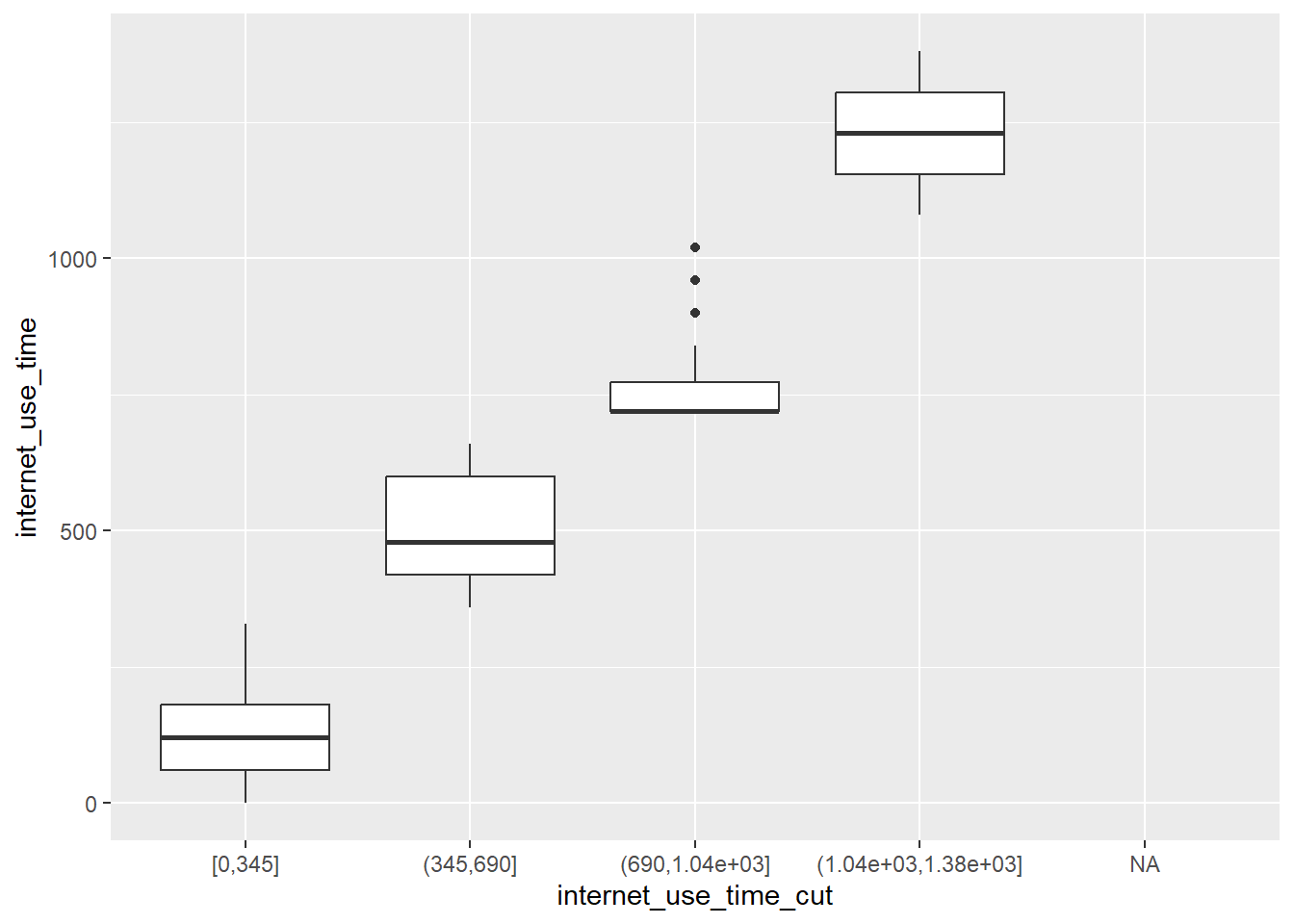
5.1.2 Discretizing data
Sometimes it makes sense to discretize data, i.e., convert it to less categories. Below we create a new variable based on internet_use_time with four categories:
Below we use a loop to explore whether our data contains factor variables that have many values. Subsequently, we could delete them.
# Identify factors with too many levels# Identify factors with too many levelsfor(i innames(data)){if(!is.factor(data %>%pull(i))) next# Skip non-factorsif(length(levels(data %>%pull(i)))<9) next# Skip if levels < Xcat("\n\n\n",i,"\n") # Print variableprint(levels(data %>%pull(i))) # Print levelsSys.sleep(0) # Increase if many variables }
Afterwards we could decide to drop those variables or to recode them in some fashion.
6 All the code
# install.packages(pacman)pacman::p_load(tidyverse, tidymodels, knitr, kableExtra, DataExplorer, visdat, naniar, skimr, modelsummary)load(file ="www/data/data_ess.Rdata")# Select a few variables for illustrationdata <- data %>%select(respondent_id, life_satisfaction, age, education, internet_use_frequency, religion)datasummary_skim(data, type ="numeric")datasummary_skim(data, type ="categorical")recipe1 <-# Store recipe in object recipe 1# Step 1: Define formula and data# "." -> all predictorsrecipe(life_satisfaction ~ ., data = data) %>%# Define formula; use "." to select all predictors in dataset# Step 2: Define rolesupdate_role(respondent_id, new_role ="ID") %>%# Define ID variable# Step 3: Handle Missing Valuesstep_naomit(all_predictors()) %>%# Step 4: Feature Scaling (if applicable)# Assuming you have numerical features that need scalingstep_normalize(all_numeric_predictors()) %>%# Step 5: Add polynomials for all numeric predictorsstep_poly(all_numeric_predictors(), degree =2, keep_original_cols =TRUE,options =list(raw =TRUE)) %>%# Step 6: Encode Categorical Variables (AFTER TREATING OTHER NUMERIC VARIABLES)step_dummy(all_nominal_predictors(), one_hot =TRUE)# see also step_ordinalscore() to convert to numeric# Inspect the recipe recipe1# Now you can apply the recipe to your datadata_preprocessed <-prep(recipe1, data)# Access and inspect the preprocessed data with $View(data_preprocessed$template)skim(data_preprocessed$template)# Below we simply use one dataset (and do not split)dim(data)names(data)# Define a recipe for preprocessing (taken from above) recipe1 <-recipe(life_satisfaction ~ ., data = data) %>%# Define formula; update_role(respondent_id, new_role ="ID") %>%# Define ID variablestep_unknown(religion) %>%# Change missings to unknownstep_naomit(all_predictors()) %>%step_normalize(all_numeric_predictors()) %>%step_poly(all_numeric_predictors(), degree =2, keep_original_cols =TRUE,options =list(raw =TRUE)) %>%step_dummy(all_nominal_predictors(), one_hot =TRUE)# Define a model model1 <-linear_reg() %>%# linear modelset_engine("lm") %>%# lm engineset_mode("regression") # regression problem# Define a workflow workflow1 <-workflow() %>%# create empty workflowadd_recipe(recipe1) %>%# add recipeadd_model(model1) # add model workflow1 # Inspect# Train the model (on all the data.. no split here..) fit1 <-fit(workflow1, data = data)# Print summary of the trained model fit1# install.packages(pacman)pacman::p_load(tidyverse, tidymodels, naniar, knitr, kableExtra, DataExplorer, visdat)load(file ="www/data/data_ess.Rdata")# install.packages(pacman)pacman::p_load(tidyverse, tidymodels, naniar, knitr, kableExtra, DataExplorer, visdat)# Load the .RData file into Rload(url(sprintf("https://docs.google.com/uc?id=%s&export=download","173VVsu9TZAxsCF_xzBxsxiDQMVc_DdqS")))# Subset variablesdata <- data %>%select(respondent_id, life_satisfaction, age, education, internet_use_frequency, religion, trust_people)# Extract data with missing outcome data_missing_outcome <- data %>%filter(is.na(life_satisfaction))dim(data_missing_outcome)# Omit individuals with missing outcome from data data <- data %>%drop_na(life_satisfaction) # ?drop_nadim(data)# Split the data into training and test dataset.seed(1234) data_split <-initial_split(data, prop =0.80) data_split # Inspect# Extract the two datasets data_train <-training(data_split) data_test <-testing(data_split) # Do not touch until the end!# AFTER SPLIT# Define a recipe for preprocessing (taken from above) recipe1 <-recipe(life_satisfaction ~ ., data = data_train) %>%# Define formula; update_role(respondent_id, new_role ="ID") %>%# Define ID variablestep_impute_mean(all_numeric_predictors()) %>%step_naomit(all_predictors()) %>%step_normalize(all_numeric_predictors()) %>%step_poly(all_numeric_predictors(), degree =1, keep_original_cols =TRUE,options =list(raw =TRUE)) %>%step_dummy(all_nominal_predictors(), one_hot =TRUE) recipe1# Define a model model1 <-linear_reg() %>%# linear modelset_engine("lm") %>%# lm engineset_mode("regression") # regression problem# Define a workflow workflow1 <-workflow() %>%# create empty workflowadd_recipe(recipe1) %>%# add recipeadd_model(model1) # add model # Fit the workflow (including recipe and model) fit1 <- workflow1 %>%fit(data = data_train)# Training data: Add predictions & calculate metricsaugment(fit1, data_train) %>%metrics(truth = life_satisfaction, estimate = .pred)# Test data: Add predictions & calculate metricsaugment(fit1, data_test) %>%metrics(truth = life_satisfaction, estimate = .pred)# Dropping datadata <- data %>%drop_na(life_satisfaction) %>%# Drop missing on outcomeselect(where(~mean(is.na(.)) <0.5)) # select features with less than X % missing# data_listwise <- data %>% na.omit() # Listwise deletion (Be careful!)# Dropping datadata <- data %>%mutate(internet_use_time_cut =cut_interval(internet_use_time, 4))ggplot(data = data,aes(x = internet_use_time_cut,y = internet_use_time)) +geom_boxplot()# Identify factors with too many levels# Identify factors with too many levelsfor(i innames(data)){if(!is.factor(data %>%pull(i))) next# Skip non-factorsif(length(levels(data %>%pull(i)))<9) next# Skip if levels < Xcat("\n\n\n",i,"\n") # Print variableprint(levels(data %>%pull(i))) # Print levelsSys.sleep(0) # Increase if many variables }labs = knitr::all_labels()ignore_chunks <- labs[str_detect(labs, "exclude|setup|solution|get-labels")]labs =setdiff(labs, ignore_chunks)
References
Garcı́a, Salvador, Julián Luengo, and Francisco Herrera. 2015. Data Preprocessing in Data Mining. Springer International Publishing.
James, Gareth, Daniela Witten, Trevor Hastie, and Robert Tibshirani. 2013. An Introduction to Statistical Learning: With Applications in R. Springer Texts in Statistics. Springer.
Footnotes
Examples are: predictor (independent variables), response, and case weight. This is meant to be open-ended and extensible.↩︎
These are synonymous with features in machine learning. Variables that have predictor roles would automatically be main effect terms.↩︎
which is carried along but not used in the model↩︎