| respondent_id | life_satisfaction | country | unemployed_active | unemployed | education | news_politics_minutes |
|---|---|---|---|---|---|---|
| 10005 | 10 | FR | 0 | 0 | 3 | 50 |
| 10007 | 7 | FR | 0 | 0 | 5 | 120 |
| 10011 | 7 | FR | 0 | 0 | 3 | 5 |
| 10022 | 5 | FR | 0 | 0 | 0 | 75 |
| 10025 | 7 | FR | 0 | 0 | 3 | 60 |
| 10050 | 10 | FR | 0 | 0 | 2 | 30 |
| 10069 | 8 | FR | 0 | 0 | 2 | 60 |
| 10092 | 8 | FR | 0 | 0 | 2 | 90 |
| 10096 | 6 | FR | 0 | 0 | 4 | 30 |
| 10118 | 9 | FR | 0 | 0 | 1 | 30 |
Regression: Linear model
Learning outcomes/objective: Learn…
- …how the linear regression model works from a predictive perspective.
- …in which situations we can use it for predictions.
- …how to use linear regression as a ML model in R with tidymodels.
Sources: #TidyTuesday and tidymodels
1 Predicting Life Satisfaction: The data
Table 1 depicts the first rows/columns of the dataset (European Social Survey 10, France) we use.
- Q: Why might anyone be interested in builing a predictive model for life satisfaction?
2 Linear model: Equation (1)
- Linear Model = LM = Linear regression model
- Aim (normally)
- Model (also understand) relationship between outcome variable (output) und 1+ explanatory variables (features)
- But a popular machine learning model as well (Q: Why?)!1
- Q: How many parameters can we find in the equation above and which ones?
- Q: What is \(\color{red}{\varepsilon}_{i}\)?
- Q: How do we also call \(\color{blue}{\beta_{0}}\), \(\color{orange}{\beta _{1}}\) and \(\color{orange}{\beta _{2}}\) in the ML context?
3 Linear model: Equation (2)
Q: Why is the linear model called “linear” model?
Important:
- Variable values (e.g., \(y_{i}\) or \(x_{1,i}\)) vary, parameter values (e.g., \(\boldsymbol{\color{blue}{\beta_{0}}}\)) are constant across rows
- Predictions \(\color{green}{\widehat{y}_{i}}\) varies across units
| Name | \(Lifesatisfaction\) \(y_{i}\) |
\(\boldsymbol{\color{blue}{\beta_{0}}}\) | \(\boldsymbol{\color{orange}{\beta_{1}}}\) | \(Unemployed\) \(x_{1,i}\) |
\(\boldsymbol{\color{orange}{\beta_{2}}}\) | \(Education\) \(x_{2,i}\) |
\(\boldsymbol{\color{red}{\varepsilon_{i}}}\) | \(\color{green}{\widehat{y}_{i}}\) |
|---|---|---|---|---|---|---|---|---|
| Samuel | 7 | ? | ? | 0 | ? | 5 | ? | ? |
| Ruth | 8 | ? | ? | 1 | ? | 3 | ? | ? |
| William | 2 | ? | ? | 0 | ? | 3 | ? | ? |
| .. | .. | .. | .. | .. | .. | .. | .. | .. |
4 Linear model: Visualization
- Figure 1 visualizes the distribution of our data and a linear model (3 variables!) that we fit to the data
- Lifesatisfactioni = b0 + b1Unemployed_activei + b1Educationi + \(\epsilon\)i
- The plane in Figure 1 is no exact model of the data
- Admissible model must be consistent with all the data points
- Plane cannot be model, unless it exactly fits all the data points
- Hence, error term, \(\varepsilon_{i}\), must be included in the model equation, so that it is consistent with all data points
- Q1: Predictive accuracy: Would you say our model does a good job at predicting life satisfaction?
- Q2: Looking at the graph what could a more flexible model look like?
- Q3: Are the coefficients of unemployed_active and education negative or positive?
Answers
- Q1 Predictive accuracy: Hard to say. We need to calculate average error across all errors \(\varepsilon_{i}\) (in the test dataset). However, looks as if the place is quite far from a lot of observations.
- Q2 Flexible model: Potentially, a non-linear plane that adapts more to the data.
- Q3 Coefficients: Both are negative.
5 Linear model: Estimation
- Estimation = Fitting the model to the data (by adapting/finding the parameters)
- e.g. easy in case of the mean (analytical) but more difficult e.g. for linear (or other) model(s)
- Modellparameter: \(\color{orange}{\beta_{0}}\), \(\color{orange}{\beta_{1}}\) and \(\color{orange}{\beta_{2}}\)
- Ordinary Least Squares (OLS)
- Choose \(\color{orange}{\beta_{0}}\), \(\color{orange}{\beta_{1}}\) and \(\color{orange}{\beta_{2}}\) (= plane) so that the sum of the squared errors \(\color{red}{\varepsilon}_{i}\) is minimized
- Q: Why do we square the errors?
6 Linear model: Prediction
- To predict the outcome we simply plugin a unit’s feature/predictor values \(X\) into our equation
\(y_{i1} = {\color{blue}{6.42}} + {\color{orange}{-0.55}} \times x_{1i1} + {\color{orange}{0.21}} \times x_{2i1} + {\color{red}{\varepsilon}_{i1}}\)
\(7 = {\color{blue}{6.42}} + {\color{orange}{-0.55}} \times 0 + {\color{orange}{0.21}} \times 5 + {\color{red}{-0.45}} = {\color{green}{7.45}} + {\color{red}{-0.45}}\)
7 Regression (Linear model): Accuracy (1)
- Mean squared error (James et al. 2013, Ch. 2.2)
- \(MSE=\frac{1}{n}\sum_{i=1}^{n}(y_{i}- \hat{f}(x_{i}))^{2}\) (James et al. 2013, Ch. 2.2.1)
- \(y_{i}\) is \(i\)s true outcome value
- \(\hat{f}(x_{i})\) is the prediction that \(\hat{f}\) gives for the \(i\)th observation \(\hat{y}_{i}\)
- MSE is small if predicted responses are to the true responses, and large if they differ substantially
- \(MSE=\frac{1}{n}\sum_{i=1}^{n}(y_{i}- \hat{f}(x_{i}))^{2}\) (James et al. 2013, Ch. 2.2.1)
- Training MSE: MSE computed using the training data
- Test MSE: How is the accuracy of the predictions that we obtain when we apply our method to previously unseen test data?
- \(\text{Ave}(y_{0} - \hat{f}(x_{0}))^{2}\): the average squared prediction error for test observations \((y_{0},x_{0})\)
- Usually, when building a model we used a third dataset to assess accuracy, i.e., analysis (training) data, assessment (validation) data and test data
8 Regression (Linear model): Accuracy (2)
- In practice we often use the Root Mean Squared Error (RMSE) or the Mean Absolute Error (MAE) (see formulas below)
- RMSE is in same units as the dependent variable, making it more interpretable than MSE (= units squared)
- Interpretability: MAE more straightforward averaging absolute differences directly; RMSE involves squaring and square roots complicating its interpretation
- Robustness to Outliers: MAE less sensitive to outliers, treating all errors equally; RMSE emphasizes larger errors due to squaring
- R-squared measures the proportion of variance in the outcome variable that is explained by the model
- Ranges from 0 to 1, where 0 means the model explains none of the variance and 1 means the model explains all of the variance
- Calculated as the ratio of the explained variance to the total variance of the outcome variable (measure of the model’s goodness of fit)
Formulas
\[ \text{RMSE} = \sqrt{\frac{1}{n} \sum_{i=1}^{n} (y_i - \hat{y}_i)^2} \]
Where: - \(n\) is the number of observations, - \(y_i\) is the actual value of the \(i\)th observation, - \(\hat{y}_i\) is the predicted value for the \(i\)th observation, - The square root is taken after summing the squared differences and dividing by \(n\).
\[ \text{MAE} = \frac{1}{n} \sum_{i=1}^{n} |y_i - \hat{y}_i| \]
Where: - \(n\) is the number of observations, - \(y_i\) is the actual value for the \(i\)th observation, - \(\hat{y}_i\) is the predicted value for the \(i\)th observation, - The absolute value of the differences is summed up and then divided by \(n\).
9 Lab: ML Regression using a linear modeln
Learning outcomes/objective: Learn…
- …how to predict using a regression model relying on tidymodels.
Sources: #TidyTuesday and tidymodels
9.1 The data
Below we’ll use the European Social Survey (ESS) [Round 10 - 2020. Democracy, Digital social contacts] to illustrate how to use linear models for machine learning. The ESS contains different outcomes amenable to both classification and regression as well as a lot of variables that could be used as features (~580 variables). And we’ll focus on the french survey respondents.
The variables were named not so well, so we have to rely on the codebook to understand their meaning. You can find it here or on the website of the ESS.
life_satisfaction = stflife: measures life satisfaction (How satisfied with life as a whole).unemployed_active = uempla: measures unemployment (Doing last 7 days: unemployed, actively looking for job).unemployed = uempli: measures life satisfaction (Doing last 7 days: unemployed, not actively looking for job).education = eisced: measures education (Highest level of education, ES - ISCED).country = cntry: measures a respondent’s country of origin (here held constant for France).- etc.
We first import the data into R and load a few packages:
9.2 Inspecting the dataset
First we should make sure to really explore/unterstand our data. How many observations are there? How many different variables (features) are there? What is the scale of the outcome (here we focus on life satisfaction)? What are the averages etc.? What kind of units are in your dataset?
Also always inspect summary statistics for both numeric and categorical variables to get a better understanding of the data. Often such summary statistics will also reveal (coding) errors in the data. Here we take a subset because the are too many variables (>250).
Q: Does anything strike you as interesting the two tables below?
library(modelsummary)
data_summary <- data %>%
select(life_satisfaction, unemployed_active, unemployed, education, age)
datasummary_skim(data_summary, type = "numeric", output = "html")| Unique (#) | Missing (%) | Mean | SD | Min | Median | Max | ||
|---|---|---|---|---|---|---|---|---|
| life_satisfaction | 12 | 10 | 7.0 | 2.2 | 0.0 | 8.0 | 10.0 |  |
| unemployed_active | 2 | 0 | 0.0 | 0.2 | 0.0 | 0.0 | 1.0 |  |
| unemployed | 2 | 0 | 0.0 | 0.1 | 0.0 | 0.0 | 1.0 |  |
| education | 8 | 1 | 3.1 | 1.9 | 0.0 | 3.0 | 6.0 |  |
| age | 76 | 0 | 49.5 | 18.7 | 16.0 | 50.0 | 90.0 |  |
The table() function is also useful to get an overview of variables. Use the argument useNA = "always" to display potential missings.
0 1 2 3 4 5 6 7 8 9 10 <NA>
34 14 43 50 76 170 170 324 465 213 213 205
0 1 2 3 4 5 6 7 8 9 10 <NA>
0 8 5 8 3 5 24 23 28 33 12 23 26
1 2 0 3 3 11 17 16 35 32 15 22 19
2 16 5 13 16 25 54 46 56 99 40 41 43
3 4 3 12 12 20 26 30 59 96 47 45 42
4 1 1 3 6 6 25 21 50 69 32 28 29
5 1 0 1 4 1 9 12 32 42 16 14 11
6 2 0 2 5 8 15 21 63 91 50 40 33
<NA> 0 0 1 1 0 0 1 1 3 1 0 2
0 1 2 3 4 5 6 7 8 9 10 <NA>
0 0.00 0.00 0.00 0.00 0.00 0.01 0.01 0.01 0.02 0.01 0.01 0.01
1 0.00 0.00 0.00 0.00 0.01 0.01 0.01 0.02 0.02 0.01 0.01 0.01
2 0.01 0.00 0.01 0.01 0.01 0.03 0.02 0.03 0.05 0.02 0.02 0.02
3 0.00 0.00 0.01 0.01 0.01 0.01 0.02 0.03 0.05 0.02 0.02 0.02
4 0.00 0.00 0.00 0.00 0.00 0.01 0.01 0.03 0.03 0.02 0.01 0.01
5 0.00 0.00 0.00 0.00 0.00 0.00 0.01 0.02 0.02 0.01 0.01 0.01
6 0.00 0.00 0.00 0.00 0.00 0.01 0.01 0.03 0.05 0.03 0.02 0.02
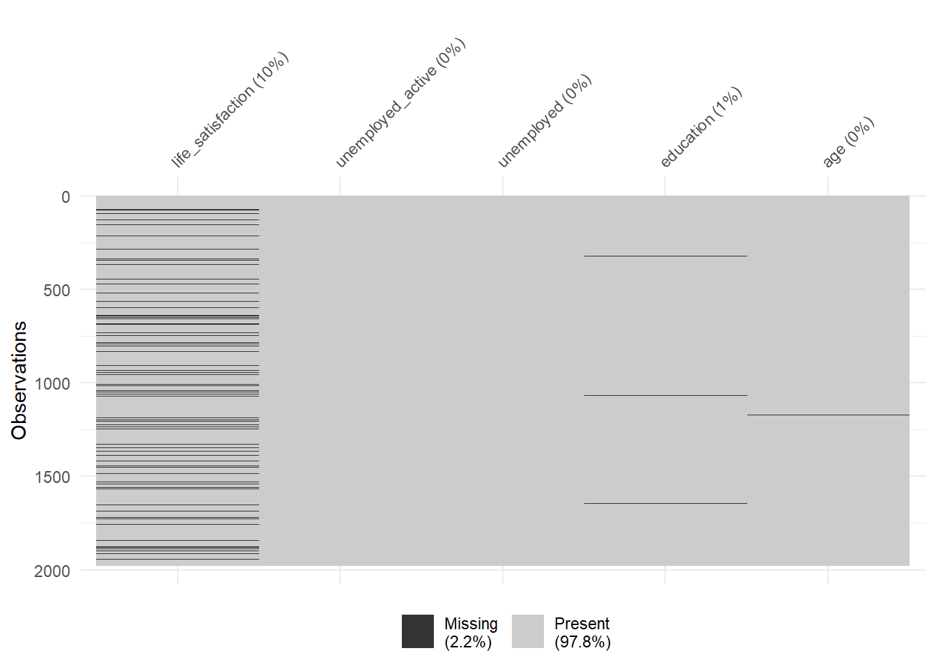
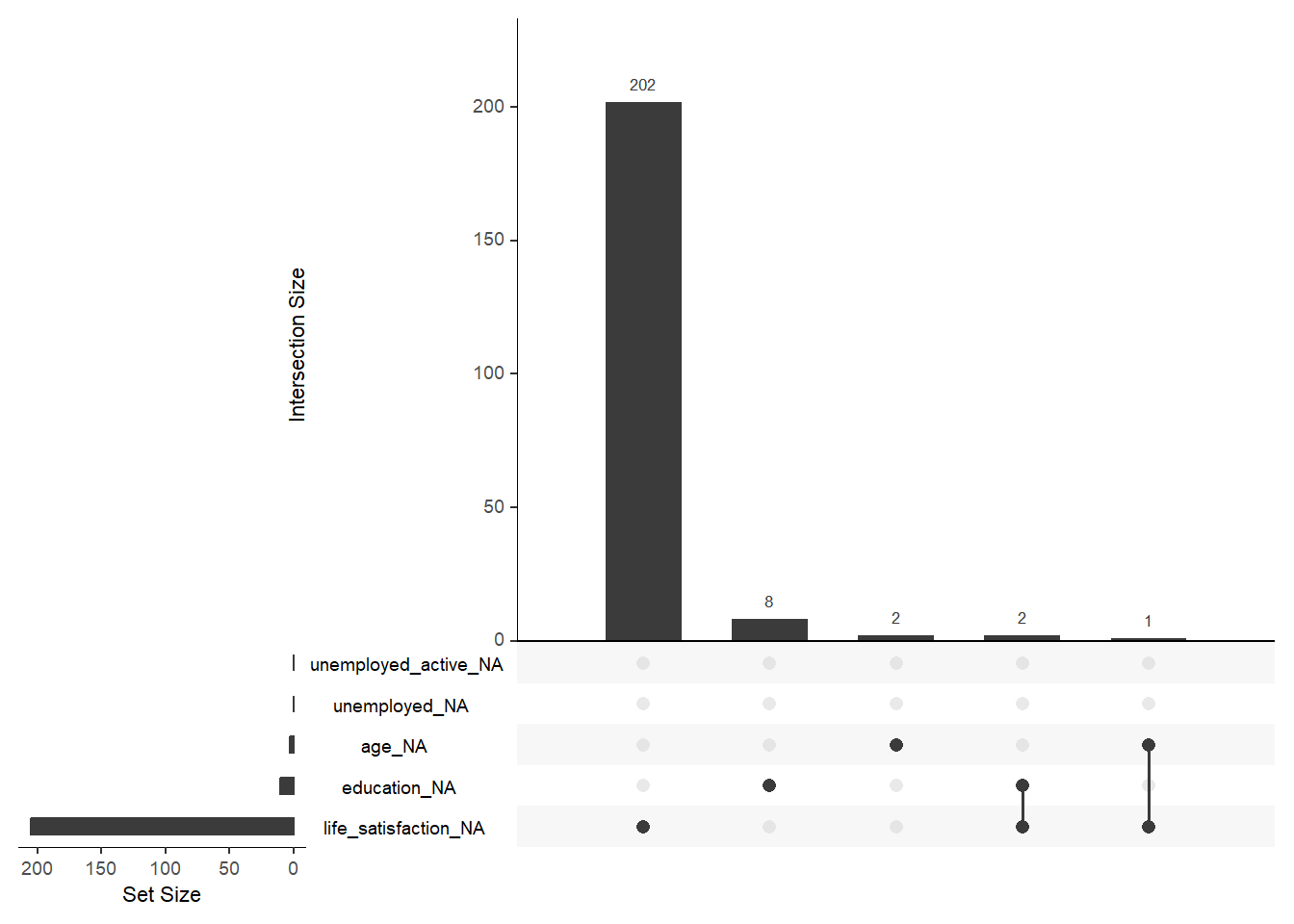
<NA> 0.00 0.00 0.00 0.00 0.00 0.00 0.00 0.00 0.00 0.00 0.00 0.00Finally, there are some helpful functions to explore missing data included in the naniar package. Here we do so for a subset of variables. Can you decode those graphs? What do they show? (for publications the design would need to be improved)
9.3 Exploring potential predictors
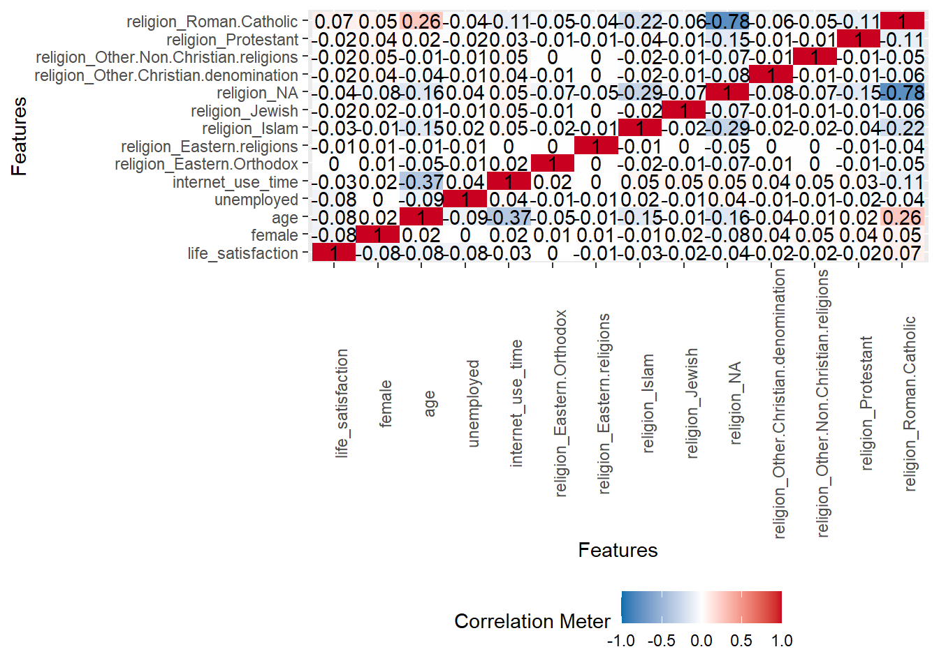
A correlation matrix can give us first hints regarding important predictors.
- Q: Can we identify anything interesting?
9.4 Building a first linear ML model
Below we estimate a simple linear machine learning model only using one split into training and test data. Beforehand we extract the subset of individuals for whom our outcome life_satisfaction is missing, store them data_missing_outcome and delete those individuals from the actual dataset data.
# Extract data with missing outcome
data_missing_outcome <- data %>% filter(is.na(life_satisfaction))
dim(data_missing_outcome)[1] 205 346# Omit individuals with missing outcome from data
data <- data %>% drop_na(life_satisfaction) # ?drop_na
dim(data)[1] 1772 346
Then we split the data into training and test data.
# Split the data into training and test data
data_split <- initial_split(data, prop = 0.80)
data_split # Inspect<Training/Testing/Total>
<1417/355/1772>
Subsequently, we estimate our linear model based on the training data. Below we just use 3 predictors:
# Fit the model
fit1 <- linear_reg() %>% # linear model
set_engine("lm") %>% # define lm package/function
set_mode("regression") %>%# define mode
fit(life_satisfaction ~ unemployed + age + education, # fit the model
data = data_train) # based on training data
fit1parsnip model object
Call:
stats::lm(formula = life_satisfaction ~ unemployed + age + education,
data = data)
Coefficients:
(Intercept) unemployed age education
6.653962 -1.363026 -0.003673 0.197203
Then, we predict our outcome in the training data and evaluate the accuracy in the training data.
# Training data: Add predictions
data_train <- augment(fit1, data_train)
head(data_train %>%
select(life_satisfaction, unemployed, age, education, .pred))# A tibble: 6 × 5
life_satisfaction unemployed age education .pred
<dbl> <dbl> <dbl> <dbl> <dbl>
1 7 0 80 2 6.75
2 1 0 58 0 6.44
3 8 0 79 4 7.15
4 9 0 76 3 6.97
5 8 0 61 6 7.61
6 6 0 33 4 7.32# A tibble: 3 × 3
.metric .estimator .estimate
<chr> <chr> <dbl>
1 rmse standard 2.17
2 rsq standard 0.0368
3 mae standard 1.67 - Q: How can we interpret the accuracy metrics? Are we happy? Or should we improve the model for the training data?
Finally, we can also predict data for the test data and evaluate the accuracy in the test data.
# Test data: Add predictions
data_test <- augment(fit1, data_test)
head(data_train %>%
select(life_satisfaction, unemployed, age, education, .pred))# A tibble: 6 × 5
life_satisfaction unemployed age education .pred
<dbl> <dbl> <dbl> <dbl> <dbl>
1 7 0 80 2 6.75
2 1 0 58 0 6.44
3 8 0 79 4 7.15
4 9 0 76 3 6.97
5 8 0 61 6 7.61
6 6 0 33 4 7.32# A tibble: 3 × 3
.metric .estimator .estimate
<chr> <chr> <dbl>
1 rmse standard 2.26
2 rsq standard 0.0401
3 mae standard 1.71 Q: The accuracy seems similar to that in the training data. What could be the reasons?
Answers
- The split training data/test data was random and both datasets are “relatively” large. And we use a very inflexible model with few features that does not adapt a lot to the training data. With a more flexible model and smaller datasets, more adaption would happen leading to better accuracy in the trainning data (but potentially worse accuracy in the test data).
If we are happy with the accuracy in the training data we could then use our model to predict the outcomes for those individuals for which we did not observe the outcome which we stored in data_missing.
# Missing outcome data predictions
data_missing_outcome <- augment(fit1, data_missing_outcome)
head(data_missing_outcome %>%
select(life_satisfaction, unemployed, age, education, .pred))# A tibble: 6 × 5
life_satisfaction unemployed age education .pred
<dbl> <dbl> <dbl> <dbl> <dbl>
1 NA 0 62 2 6.82
2 NA 0 48 0 6.48
3 NA 0 78 3 6.96
4 NA 1 53 2 5.49
5 NA 0 60 6 7.62
6 NA 0 68 6 7.599.4.1 Visualizing predictions & errors
It is often insightful to visualize a MLM’s predictions, e..g, exploring whether our predictions are better or worse for certain population subsets (e.g., the young). In other words, whether the model works better/worse across groups. Below we take data_test from above (which includes the predictions) and calculate the errors and the absolute errors.
data_test <- data_test %>%
mutate(errors = life_satisfaction - .pred, # calculate errors
errors_abs = abs(errors)) %>% # calculate absolute errors
select(life_satisfaction, unemployed, age, education, .pred, errors, errors_abs) # only keep relevant variables
head(data_test)# A tibble: 6 × 7
life_satisfaction unemployed age education .pred errors errors_abs
<dbl> <dbl> <dbl> <dbl> <dbl> <dbl> <dbl>
1 9 0 36 4 7.31 1.69 1.69
2 8 0 44 6 7.68 0.324 0.324
3 8 0 53 2 6.85 1.15 1.15
4 6 0 24 3 7.16 -1.16 1.16
5 3 0 62 2 6.82 -3.82 3.82
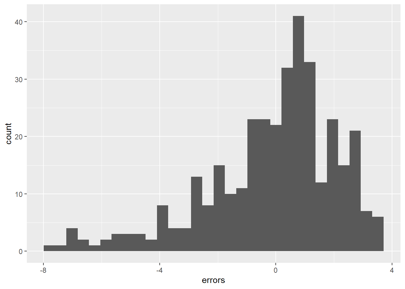
6 8 0 42 6 7.68 0.317 0.317Figure 2 visualizes the variation of errors in a histogram. What can we see?
In Figure 3 we visualize the errors as a function of covariates/predictors after discretizing and factorizing the numeric variables.
Q: What can we observe? Why is the prediction error seemingly higher for the unemployed (= 1)?
# Visualize errors and predictors
library(patchwork)
data_plot <- data_test %>%
select(errors, errors_abs, unemployed, age, education) %>%
mutate(unemployed = factor(unemployed, ordered = FALSE),
education = factor(education, ordered = TRUE),
age = cut_interval(age, 8))
p1 <- ggplot(data = data_plot, aes(y = errors, x = unemployed)) +
geom_boxplot()
p2 <- ggplot(data = data_plot, aes(y = errors, x = education)) +
geom_boxplot()
p3 <- ggplot(data = data_plot, aes(y = errors, x = age)) +
geom_boxplot() +
theme(axis.text.x = element_text(angle = 30, hjust = 1))
p1 + p2 + p3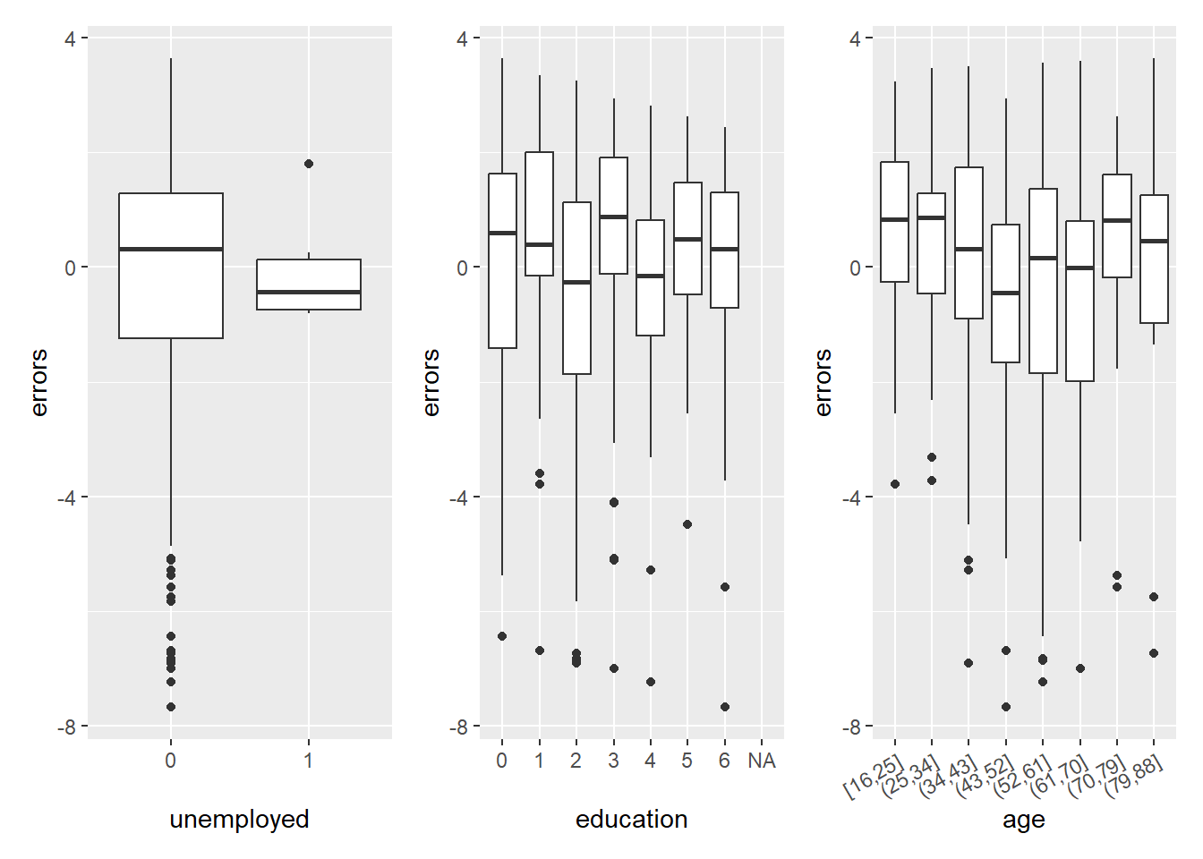
9.5 Exercise: Enhance simple linear model
- Use the code below to load the data.
- In the next chunk you find the code we used above to built our first predictive model for our outcome
life_satisfaction. Please use the code and add further predictors to the model (maybe evenage^2). Can you find a model with better accuracy in the training data (and better or worse accuracy in the test data?
# Extract data with missing outcome
data_missing_outcome <- data %>% filter(is.na(life_satisfaction))
dim(data_missing_outcome)
# Omit individuals with missing outcome from data
data <- data %>% drop_na(life_satisfaction) # ?drop_na
dim(data)
# Split the data into training and test data
data_split <- initial_split(data, prop = 0.80)
data_split # Inspect
# Extract the two datasets
data_train <- training(data_split)
data_test <- testing(data_split) # Do not touch until the end!
# Fit the model
fit1 <- linear_reg() %>% # linear model
set_engine("lm") %>% # define lm package/function
set_mode("regression") %>%# define mode
fit(life_satisfaction ~ unemployed + age + education + religion, # fit the model
data = data_train) # based on training data
fit1
# summary(fit1$fit) # Access fit within the object
# Training data: Add predictions
data_train %>% augment(fit1)
data_train %>%
augment(fit1) %>%
select(life_satisfaction, unemployed, age, education, .pred) %>%
head()
# Training data: Metrics
data_train %>%
augment(fit1) %>%
metrics(truth = life_satisfaction, estimate = .pred)
# Test data: Add predictions
data_test %>% augment(fit1)
data_test %>%
augment(fit1) %>%
select(life_satisfaction, unemployed, age, education, .pred) %>%
head()
# Test data: Metrics
data_test %>%
augment(fit1) %>%
metrics(truth = life_satisfaction, estimate = .pred)9.6 Appendix: Same but trying to avoid tidymodels
# install.packages(pacman)
pacman::p_load(tidyverse,
tidymodels,
DataExplorer,
vis_dat,
naniar) # Naniar include the gg_miss_upset function
# Load the .RData file into R
load(url(sprintf("https://docs.google.com/uc?id=%s&export=download",
"173VVsu9TZAxsCF_xzBxsxiDQMVc_DdqS")))
# Extract data with missing outcome
data_missing_outcome <- data %>% filter(is.na(life_satisfaction))
dim(data_missing_outcome)
# Omit individuals with missing outcome from data
data <- data %>% drop_na(life_satisfaction) # ?drop_na
dim(data)
# Split the data into training and test data
randomized_vector <- as.logical(rbinom(n = nrow(data), size = 1, prob = 0.2))
table(randomized_vector)
data_split <- initial_split(data, prop = 0.80)
data_split # Inspect
# Extract the two datasets
data_train <- data[!randomized_vector,]
data_test <- data[randomized_vector,]
dim(data_train)
dim(data_test)
# Fit the model
fit1 <- lm(life_satisfaction ~ unemployed + age + education + religion,
data = data_train)
# Training data: Add predictions
data_train$.pred <- predict(fit1, data_train)
head(data_train %>%
select(life_satisfaction, unemployed, age, education, .pred))
# Training data: Metrics
data_train %>%
metrics(truth = life_satisfaction, estimate = .pred)
# Test data: Add predictions
data_test$.pred <- predict(fit1, data_test)
head(data_test %>%
select(life_satisfaction, unemployed, age, education, .pred))
# After that calculate metrics for both training and test data!
# e.g., RMSE
sqrt(mean((data_train$life_satisfaction - data_train$.pred)^2, na.rm = TRUE))
sqrt(mean((data_test$life_satisfaction - data_test$.pred)^2, na.rm = TRUE))10 All the code
# namer::unname_chunks("03_01_predictive_models.qmd")
# namer::name_chunks("03_01_predictive_models.qmd")
options(scipen=99999)
#| echo: false
library(tidyverse)
library(lemon)
library(knitr)
library(kableExtra)
library(dplyr)
library(plotly)
library(randomNames)
library(stargazer)
library(haven)
load(file = "www/data/data_ess.Rdata")
data_table <- data %>%
slice(1:10) %>%
select(1:7)
data_table %>%
kable(format = "html",
escape=FALSE,
align=c(rep("l", 1), "c", "c")) %>%
kable_styling(font_size = 16)
data_plot <- data %>%
#sample_n(2000) %>% # SAMPLE!
mutate(outcome = life_satisfaction,
feature1 = unemployed_active,
feature2 = education) %>%
select(outcome, feature1, feature2) %>%
na.omit() %>%
mutate(feature1_jitter = jitter(feature1, factor = 0.3),
feature2_jitter = jitter(feature2),
outcome_jitter = jitter(outcome))
feature1 = seq(min(data_plot$feature1), max(data_plot$feature1), by = 1)
feature2 = seq(min(data_plot$feature2), max(data_plot$feature2), by = 1)
lm1 <- lm(outcome ~ feature1 + feature2, data = data_plot)
# summary(lm1)
data_new <- data %>%
filter(respondent_id %in% c(10007, 10405, 10412)) %>%
select(respondent_id, life_satisfaction, unemployed_active, education) %>%
mutate(outcome = life_satisfaction,
feature1 = unemployed_active,
feature2 = education)
data_new <- bind_cols(data_new,
y_hat = predict(lm1, newdata = data_new),
epsilon = data_new$life_satisfaction - predict(lm1, newdata = data_new))
data_new <- bind_cols(Name = c("Samuel", "Ruth", "William"),
data_new) %>%
select(-respondent_id)
coefficients <- coef(lm1)
b0 <- round(coefficients[1],2)
b1 <- round(coefficients[2],2)
b2 <- round(coefficients[3],2)
y_i1 <- round(data_new %>% filter(Name == "Samuel") %>% pull(life_satisfaction),2)
x1_i1 <- round(data_new %>% filter(Name == "Samuel") %>% pull(unemployed_active),2)
x2_i1 <- round(data_new %>% filter(Name == "Samuel") %>% pull(education),2)
error_i1 <- round(data_new %>% filter(Name == "Samuel") %>% pull(epsilon),2)
y_hat_i1 <- round(data_new %>% filter(Name == "Samuel") %>% pull(y_hat),2)
y_i2 <- round(data_new %>% filter(Name == "Ruth") %>% pull(life_satisfaction),2)
x1_i2 <- round(data_new %>% filter(Name == "Ruth") %>% pull(unemployed_active),2)
x2_i2 <- round(data_new %>% filter(Name == "Ruth") %>% pull(education),2)
error_i2 <- round(data_new %>% filter(Name == "Ruth") %>% pull(epsilon),2)
y_hat_i2 <- round(data_new %>% filter(Name == "Ruth") %>% pull(y_hat),2)
y_i3 <- round(data_new %>% filter(Name == "William") %>% pull(life_satisfaction),2)
x1_i3 <- round(data_new %>% filter(Name == "William") %>% pull(unemployed_active),2)
x2_i3 <- round(data_new %>% filter(Name == "William") %>% pull(education),2)
error_i3 <- round(data_new %>% filter(Name == "William") %>% pull(epsilon),2)
y_hat_i3 <- round(data_new %>% filter(Name == "William") %>% pull(y_hat),2)
grid_wide <-
expand_grid(feature1 = feature1,
feature2 = feature2) %>%
mutate(outcome_pred_lm1 = predict(lm1, newdata = data.frame(feature1, feature2))) %>%
pivot_wider(names_from = feature2,
values_from = outcome_pred_lm1) %>%
select(-1) %>% # kick the name's column out
as.matrix()
plot_ly(data_plot,
x = ~ feature1_jitter,
y = ~ feature2_jitter,
z = ~ outcome_jitter,
type = "scatter3d",
marker = list(color = '#000000',
size = 2,
opacity = 0.5,
symbol = 'circle',
line = list(color = '#000000',
width = 4)),
hoverinfo = "text",
text = paste(data_plot$Name,
"<br>Unemployed_active: ", data_plot$feature1,
"<br>Education: ", data_plot$feature2,
"<br>Lifesatisfaction: ", data_plot$outcome,
sep=""),
height = 600) %>%
add_trace(z = grid_wide,
x = rep(feature1, each = length(feature2)) %>% matrix(nrow = length(feature1),
ncol = length(feature2),
byrow = TRUE),
y = rep(feature2, length(feature1)) %>% matrix(nrow = length(feature1),
ncol = length(feature2),
byrow = TRUE),
type = "surface",
showscale=FALSE,
colorscale = list(c(0,1),
c("rgb(107,255,184)",
"rgb(0,124,90)"))) %>%
layout(scene = list(aspectratio = list(x=0.5, y=1, z=1),
xaxis = list(title = 'Unemployed_active',
tickvals = c(0,1),
range = c(0,1)),
yaxis = list(title = 'Education',
tickvals = seq(0,7,1),
range = c(0,7)),
zaxis = list(title = 'Life satisfaction',
tickvals = seq(0,10,1),
range = c(0,10)),
camera = list(center = list(z = -0.2))),
showlegend = FALSE,
legend = list(x = 0.77, y = 0.95),
title = "Joint distribution + Linear Model: <br> Life satisfaction, Unemployment and Education")
# install.packages(pacman)
pacman::p_load(tidyverse,
tidymodels,
knitr,
kableExtra,
DataExplorer,
visdat,
naniar,
patchwork)
load(file = "www/data/data_ess.Rdata")
# install.packages(pacman)
pacman::p_load(tidyverse,
               tidymodels,
               DataExplorer,
               vis_dat,
               naniar,
               patchwork) # Naniar include the gg_miss_upset function

# Load the .RData file into R
load(url(sprintf("https://docs.google.com/uc?id=%s&export=download",
                         "173VVsu9TZAxsCF_xzBxsxiDQMVc_DdqS")))
#nrow(data)
#ncol(data)
dim(data)
# str(data)
# glimpse(data)
# skimr::skim(data)
library(modelsummary)
data_summary <- data %>%
  select(life_satisfaction, unemployed_active, unemployed, education, age)
datasummary_skim(data_summary, type = "numeric", output = "html")
# datasummary_skim(data_summary, type = "categorical", output = "html")
table(data$life_satisfaction, useNA = "always")
table(data$education, data$life_satisfaction, useNA = "always")
round(prop.table(table(data$education,
                       data$life_satisfaction, useNA = "always")),2)
vis_miss(data %>%
                select(life_satisfaction,
                       unemployed_active,
                       unemployed,
                       education,
                       age))
gg_miss_upset(data %>%
                select(life_satisfaction,
                       unemployed_active,
                       unemployed,
                       education,
                       age), nsets = 10, nintersects = 10)
plot_correlation(data %>% dplyr::select(life_satisfaction, female,
                                        age, unemployed,
                                        internet_use_time, religion),
                 cor_args = list("use" = "pairwise.complete.obs"))
# Extract data with missing outcome
  data_missing_outcome <- data %>% filter(is.na(life_satisfaction))
  dim(data_missing_outcome)
# Omit individuals with missing outcome from data
  data <- data %>% drop_na(life_satisfaction) # ?drop_na
  dim(data)
# Split the data into training and test data
  data_split <- initial_split(data, prop = 0.80)
  data_split # Inspect
# Extract the two datasets
  data_train <- training(data_split)
  data_test <- testing(data_split) # Do not touch until the end!
# Fit the model
  fit1 <- linear_reg() %>% # linear model
        set_engine("lm") %>% # define lm package/function
        set_mode("regression") %>%# define mode
        fit(life_satisfaction ~ unemployed + age + education, # fit the model
        data = data_train) # based on training data
  fit1
# summary(fit1$fit) # Access fit within the object
# Training data: Add predictions
  data_train <- augment(fit1, data_train)

  head(data_train %>%
      select(life_satisfaction, unemployed, age, education, .pred))
# Training data: Metrics
  data_train %>%
      metrics(truth = life_satisfaction, estimate = .pred)
# Test data: Add predictions
  data_test <- augment(fit1, data_test)

  head(data_train %>%
      select(life_satisfaction, unemployed, age, education, .pred))
# Test data: Metrics
  data_test %>%
      metrics(truth = life_satisfaction, estimate = .pred)
# Missing outcome data predictions
  data_missing_outcome <- augment(fit1, data_missing_outcome)

  head(data_missing_outcome %>%
      select(life_satisfaction, unemployed, age, education, .pred))
data_test <- data_test %>%
  mutate(errors = life_satisfaction - .pred, # calculate errors
         errors_abs = abs(errors)) %>% # calculate absolute errors
  select(life_satisfaction, unemployed, age, education, .pred, errors, errors_abs) # only keep relevant variables
head(data_test)
# Visualize errors and predictors
ggplot(data = data_test,
       aes(x = errors)) +
  geom_histogram()
# Visualize errors and predictors
library(patchwork)
data_plot <- data_test %>%
  select(errors, errors_abs, unemployed, age, education) %>%
  mutate(unemployed = factor(unemployed, ordered = FALSE),
         education = factor(education, ordered = TRUE),
         age = cut_interval(age, 8))


p1 <- ggplot(data = data_plot, aes(y = errors, x = unemployed)) +
  geom_boxplot()
p2 <- ggplot(data = data_plot, aes(y = errors, x = education)) +
  geom_boxplot()
p3 <- ggplot(data = data_plot, aes(y = errors, x = age)) +
      geom_boxplot() +
      theme(axis.text.x = element_text(angle = 30, hjust = 1))

p1 + p2 + p3
# install.packages(pacman)
  pacman::p_load(tidyverse,
                 tidymodels,
                 DataExplorer,
                 vis_dat,
                 naniar) # Naniar include the gg_miss_upset function

# Load the .RData file into R
  load(url(sprintf("https://docs.google.com/uc?id=%s&export=download",
                           "173VVsu9TZAxsCF_xzBxsxiDQMVc_DdqS")))
# Extract data with missing outcome
  data_missing_outcome <- data %>% filter(is.na(life_satisfaction))
  dim(data_missing_outcome)

# Omit individuals with missing outcome from data
  data <- data %>% drop_na(life_satisfaction) # ?drop_na
  dim(data)


# Split the data into training and test data
  data_split <- initial_split(data, prop = 0.80)
  data_split # Inspect

# Extract the two datasets
  data_train <- training(data_split)
  data_test <- testing(data_split) # Do not touch until the end!

# Fit the model
  fit1 <- linear_reg() %>% # linear model
        set_engine("lm") %>% # define lm package/function
        set_mode("regression") %>%# define mode
        fit(life_satisfaction ~ unemployed + age + education + religion, # fit the model
        data = data_train) # based on training data
  fit1
  # summary(fit1$fit) # Access fit within the object


# Training data: Add predictions
  data_train %>% augment(fit1)

  data_train %>%
    augment(fit1) %>%
      select(life_satisfaction, unemployed, age, education, .pred) %>%
          head()

# Training data: Metrics
   data_train %>%
      augment(fit1) %>%
        metrics(truth = life_satisfaction, estimate = .pred)


# Test data: Add predictions
  data_test %>% augment(fit1)

  data_test %>%
    augment(fit1) %>%
      select(life_satisfaction, unemployed, age, education, .pred) %>%
          head()

# Test data: Metrics
   data_test %>%
      augment(fit1) %>%
        metrics(truth = life_satisfaction, estimate = .pred)
# install.packages(pacman)
pacman::p_load(tidyverse,
               tidymodels,
               DataExplorer,
               vis_dat,
               naniar) # Naniar include the gg_miss_upset function

# Load the .RData file into R
load(url(sprintf("https://docs.google.com/uc?id=%s&export=download",
                         "173VVsu9TZAxsCF_xzBxsxiDQMVc_DdqS")))

# Extract data with missing outcome
  data_missing_outcome <- data %>% filter(is.na(life_satisfaction))
  dim(data_missing_outcome)

# Omit individuals with missing outcome from data
  data <- data %>% drop_na(life_satisfaction) # ?drop_na
  dim(data)


# Split the data into training and test data
  randomized_vector <- as.logical(rbinom(n = nrow(data), size = 1, prob = 0.2))
  table(randomized_vector)


  data_split <- initial_split(data, prop = 0.80)
  data_split # Inspect

# Extract the two datasets
  data_train <- data[!randomized_vector,]
  data_test <- data[randomized_vector,]
  dim(data_train)
  dim(data_test)

# Fit the model
  fit1 <- lm(life_satisfaction ~ unemployed + age + education + religion,
             data = data_train)


# Training data: Add predictions
  data_train$.pred <- predict(fit1, data_train)

  head(data_train %>%
         select(life_satisfaction, unemployed, age, education, .pred))

# Training data: Metrics
 data_train %>%
    metrics(truth = life_satisfaction, estimate = .pred)


# Test data: Add predictions
  data_test$.pred <- predict(fit1, data_test)

  head(data_test %>%
         select(life_satisfaction, unemployed, age, education, .pred))


  # After that calculate metrics for both training and test data!
  # e.g., RMSE
  sqrt(mean((data_train$life_satisfaction - data_train$.pred)^2, na.rm = TRUE))
  sqrt(mean((data_test$life_satisfaction - data_test$.pred)^2, na.rm = TRUE))
labs = knitr::all_labels()
ignore_chunks <- labs[str_detect(labs, "exclude|setup|solution|get-labels")]
labs = setdiff(labs, ignore_chunks)References
James, Gareth, Daniela Witten, Trevor Hastie, and Robert Tibshirani. 2013. An Introduction to Statistical Learning: With Applications in R. Springer Texts in Statistics. Springer.
Footnotes
Areas: Predict housing prices; predict stock prices; sales forecasting etc. generally areas with a lot of data (that require speed) & areas that require interpretability & sometimes are with few data points -> needs non-flexible model!↩︎