Feature selection & regularization (regression)

Learning outcomes/objective: Learn…

…about model regularization/feature selection (focus on ridge regression and lasso).
…how to implement ridge regression and lasso in R with tidymodels.
…what a tuning parameter can be used for (\(\lambda\) in ridge regression/lasso)

Sources: James et al. (2013, Ch. 6), ISLR tidymodels labs by Emil Hvitfeldt

1 Concepts

Feature selection
- also known as variable selection, attribute selection or variable subset selection, is the process of selecting a subset of relevant features (variables, predictors) for use in model construction (Wikipedia)
Regularization
- = either choice of the model or modifications to the algorithm
- Penalizing the complexity of a model to reduce overfitting
Theory vs. algorithm feature selection
- ML largely focuses on automated selection, albeit theory may play an important role

2 Why using alternatives to least squares?

Why use another fitting procedure instead of least squares? (James et al. 2013, Ch. 6)
- Alternative fitting procedures can yield better prediction accuracy and model interpretability
Prediction Accuracy: Provided that the true relationship between the response and the predictors is approximately linear, the least squares estimates will have low bias
- If \(n \gg p\) (much larger) least squares estimates have low bias but if not possibility of overfitting
- By constraining or shrinking the estimated coefficients, we can often substantially reduce the variance at the cost of negligible increase in bias (James et al. 2013, 204)
Model Interpretability: Often some/many of the variables used in a multiple regression model are in fact not associated with the response/outcome
- Including such irrelevant variables leads to unnecessary complexity in resulting model
- Idea: remove these variables (set corresponding coefficient estimates to 0) to obtain a model that is more easily interpreted
- There are various methods to do so automatically

3 Methods for feature/variables selection

Subset selection: involves identifying subset of the \(p\) predictors that we believe to be related to the response
- Strategy: Fit a model using least squares on the reduced set of variables
- e.g., best subset selection (James et al. 2013, Ch. 6.1.1), forward/backward stepwise selection (relying on model fit) (James et al. 2013, Ch. 6.1.2)
- Tidymodels: “It’s not a huge priority since other methods (e.g. regularization) are uniformly superior methods to feature selection.” (Source)
Shrinkage: involves fitting a model involving all \(p\) predictors but shrink coefficients to zero relative to the least squares estimates
- This shrinkage (also known as regularization) has the effect of reducing variance
- Depending on what type of shrinkage is performed, some coefficients may be estimated to be exactly zero,i.e., shrinkage methods can perform variable selection
- e.g., ridge regression (James et al. 2013, Ch. 6.2.1), the lasso (James et al. 2013, Ch. 6.2.2)
Dimension reduction: involves projecting the \(p\) predictors into a M-dimensional subspace, where \(M<p\).
- Achieved by computing \(M\) different linear combinations (or projections) of the variables
- Then these \(M\) projections are used as predictors to fit a linear regression model by least squares
- e.g., principal components regression (James et al. 2013, Ch. 6.3.1), partial least squares (James et al. 2013, Ch. 6.3.2)

4 High dimensional data

“Most traditional statistical techniques for regression and classification are intended for the low-dimensional setting in which \(n\), the number of observations, is much greater than \(p\), the number of features” (James et al. 2013, 238)
“Data sets containing more features than observations are often referred to as high-dimensional. Classical approaches such as least squares linear regression are not appropriate in this setting.” (James et al. 2013, 239)
“It turns out that many of the methods seen in this chapter for fitting less flexible least squares models, such as forward stepwise selection, ridge regression, the lasso, and principal components regression, are particularly useful for performing regression in the high-dimensional setting. Essentially, these approaches avoid overfitting by using a less flexible fitting approach than least squares.” (James et al. 2013, 239)

5 Ridge regression (RR) (1)

Least squares (LS) estimator: least squares fitting procedure estimates \(\beta_{0}, \beta_{1}, ..., \beta_{p}\) using the values that minimize RSS
Ridge regression (RR): seeks coefficient estimates that fit data well (minimize RSS) + shrinkage penalty
- See formula (6.5) in (James et al. 2013, 215)
shrinkage penalty \(\lambda \sum_{j=1}^{p}\beta_{j}^{2}\) is small when \(\beta_{0}, \beta_{1}, ..., \beta_{p}\) close to zero
- penality has effect of shrinking the estimates \(\beta_{j}\) to zero
- Tuning parameter \(\lambda\) serves to control the relative impact of these two terms (RSS and shrinking penalty) on the regression coefficient estimates
  - When \(\lambda = 0\) the penalty term has no effect and ridge regression will produce least squares estimates
  - As \(\lambda \rightarrow \infty\), impact of the shrinkage penalty grows, and the ridge regression coefficient estimates will approach zero
- Penality is only applied to coefficients not the intercept
Ridge regression will produce a different set of coefficient estimates \(\hat{\beta}_{\lambda}^{R}\) for each \(\lambda\)
- Hyperparameter tuning: fit many models with different \(\lambda\)s to find the model the performs “best”

6 Ridge regression (RR) (2): Visualization

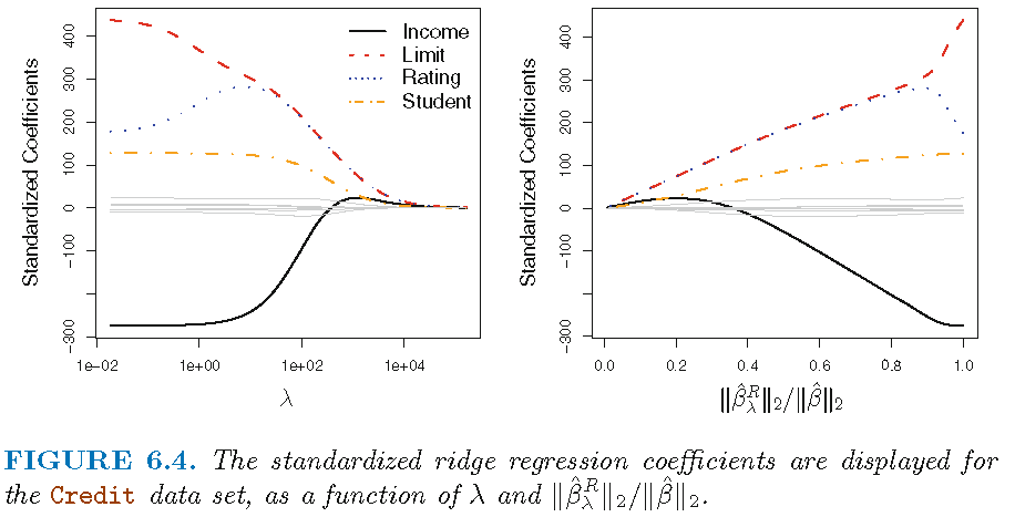
Figure 1 displays regression coefficient estimates for the Credit data (James et al. 2013, Ch. 6.2)
- Left-hand panel: each curve corresponds to the ridge regression coefficient estimate for one of the ten variables, plotted as a function of \(\lambda\)
  - to the left \(\lambda\) is essentially zero, so ridge coefficient estimates are the same as the usual least squares estimates
  - as \(\lambda\) increases, ridge coefficient estimates shrink towards zero
  - when \(\lambda\) is extremely large, all of the ridge coefficient estimates are basically zero = null model
Occasionally coefficients can increase as \(\lambda\) increases (cf. predictor “Rating”)
While standard LS coefficient estimates are scale equivalent, RR coefficients are not
- Best to apply ridge regression after standardizing the predictors (resulting in SD = 1 for all predictors and final fit independent of predictor scales)

Figure 1: Source: James et al. (2013), Ch. 6.2, Figure 6.4

7 Ridge regression (RR) (3): Why?

Why Does Ridge Regression (RR) Improve Over Least Squares (LS)?

Advantage rooted in the bias-variance trade-off
- As \(\lambda\) increases, flexibility of ridge regression fit decreases, leading to decreased variance but increased bias
  - Q: What was variance and bias again in the context of ML? (see Bias/variance trade-off)
In situations where relationship between response (outcome) and predictors is close to linear, LS estimates will have low bias but may have high variance
- \(\rightarrow\) small change in the training data can cause a large change in the LS coefficient estimates
- In particular, when number of variables \(p\) is almost as large as the number of observations \(n\) (cf. James et al. 2013, fig. 6.5), LS estimates will be extremely variable
- If \(p>n\), then LS estimates do not even have a unique solution, whereas RR can still perform well
Summary: RR works best in situations where the LS estimates have high variance

8 The Lasso

Ridge regression (RR) has one obvious disadvantage
- Unlike subset selection methods (best subset, forward stepwise, and backward stepwise selection) that select models that involve a variable subset, RR will include all \(p\) predictors in final model
- Penalty \(\lambda \sum_{j=1}^{p}\beta_{j}^{2}\) will shrink all coefficients towards zero, but no set them exactly to 0 (unless \(\lambda = \infty\))
- No problem for accuracy, but challenging for model interpretation when \(p\) is large
Lasso (least absolute shrinkage and selection operator)
- As in RR lasso shrinks the coefficient estimates towards zero but additionally…
- …its penality has effect of forcing some of the coefficient estimates to be exactly equal to zero when tuning parameter \(\lambda\) is sufficiently large (cf. James et al. 2013, Eq. 6.7, p.219)
- LASSO performs variable selection leading to easier interpretation, i.e., yields sparse models
- As in RR selecting good value of \(\lambda\) is critical

9 Comparing the Lasso and Ridge Regression

Advantage of Lasso: produces simpler and more interpretable models involving subset of predictors
However, which method leads to better prediction accuracy?
- Neither ridge regression nor lasso universally dominates the other
- Lasso works better when few predictors have significant coefficients, others have small/zero coefficients
- Ridge regression performs better with many predictors of roughly equal coefficient size
- Cross-validation helps determine the better approach for a specific data set
- Both methods can reduce variance at the cost of slight bias increase, improving prediction accuracy

10 Lab: Ridge Regression

See earlier description here (right click and open in new tab).

We first import the data into R:

library(tidymodels)
library(tidyverse)
# Load the .RData file into R
load(url(sprintf("https://docs.google.com/uc?id=%s&export=download",
                         "173VVsu9TZAxsCF_xzBxsxiDQMVc_DdqS")))

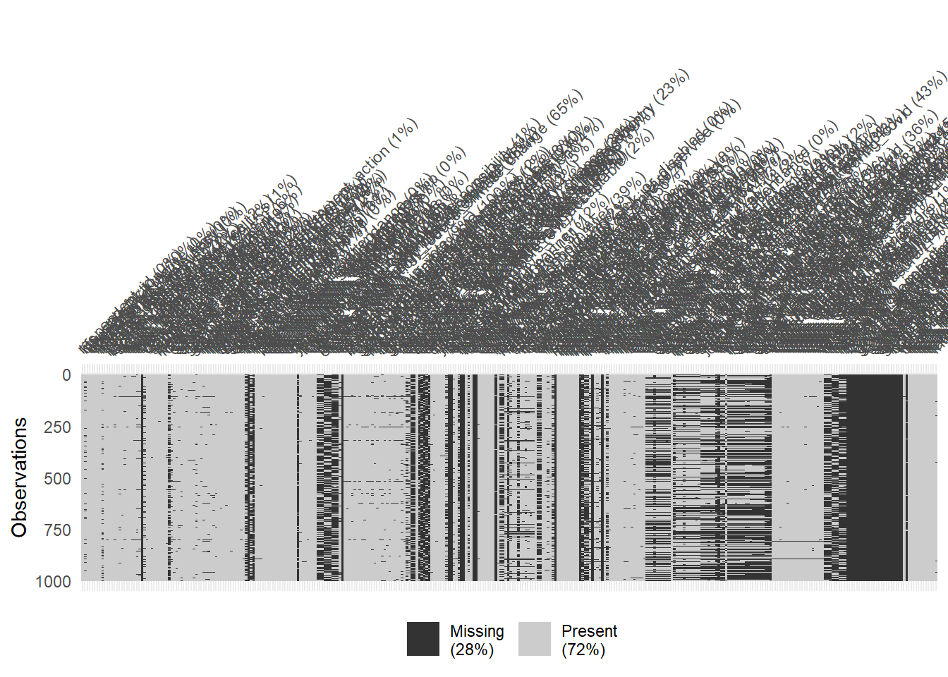
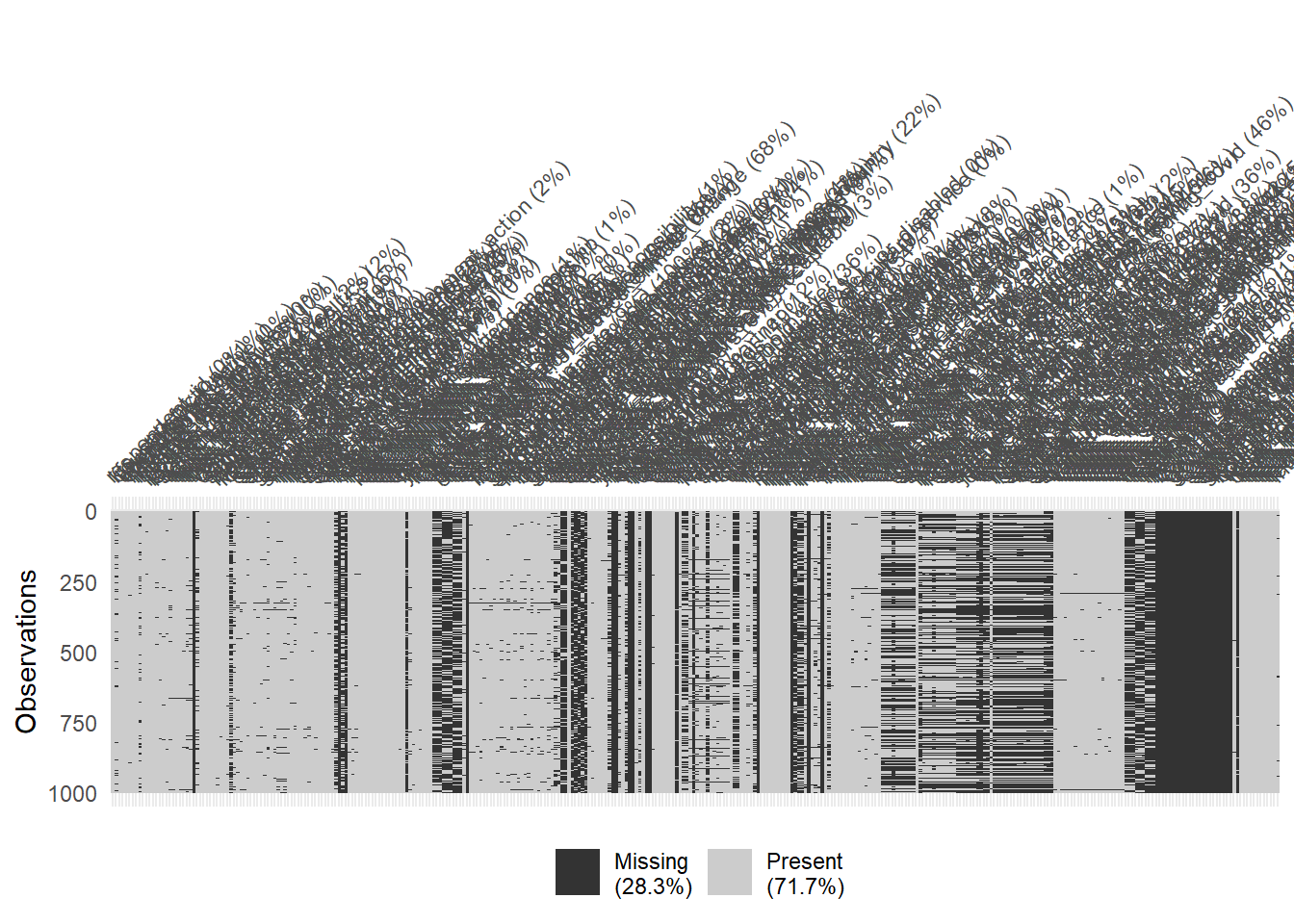
10.1 Inspecting the dataset

The dataset if relatively large with 1977 rows and 346 columns. The skim() function can be used to get a quick overview.

library(skimr)
library(naniar)

#skim(data)
nrow(data)

[1] 1977

ncol(data)

[1] 346

# Visualize missing for downsampled data
  vis_miss(data %>% sample_n(1000), warn_large_data = FALSE)

# Again: Visualize missing for downsampled data
  vis_miss(data %>% sample_n(1000), warn_large_data = FALSE)

10.2 Split the data

Below we split the data and create resampled partitions with vfold_cv() stored in an object called data_folds. Hence, we have the original data_train and data_test but also already resamples of data_train in data_folds.

# Extract data with missing outcome
  data_missing_outcome <- data %>% filter(is.na(life_satisfaction))
  dim(data_missing_outcome)

[1] 205 346

# Omit individuals with missing outcome from data
  data <- data %>% drop_na(life_satisfaction) # ?drop_na
  dim(data)

[1] 1772  346

# Split the data into training and test data
  set.seed(345)
  data_split <- initial_split(data, prop = 0.80)
  data_split # Inspect

<Training/Testing/Total>
<1417/355/1772>

# Extract the two datasets
  data_train <- training(data_split)
  data_test <- testing(data_split) # Do not touch until the end!
  
# Create resampled partitions
  data_folds <- vfold_cv(data_train, v = 5) # V-fold/k-fold cross-validation
  data_folds # data_folds now contains several resamples of our training data

#  5-fold cross-validation 
# A tibble: 5 × 2
  splits             id   
  <list>             <chr>
1 <split [1133/284]> Fold1
2 <split [1133/284]> Fold2
3 <split [1134/283]> Fold3
4 <split [1134/283]> Fold4
5 <split [1134/283]> Fold5

  # You can also try loo_cv(data_train) instead

The training data has 1417 rows, the test data has 355. The training data is further split into 10 folds.

10.3 Simple ridge regression (all in one)

Below we provide a quick example of a ridge regression (beware: below in the recipe we standardize predictors).

Arguments of glmnet linear_reg()
- mixture = 0: to specify a ridge model
  - mixture = 0 specifies only ridge regularization
  - mixture = 1 specifies only lasso regularization
  - Setting mixture to a value between 0 and 1 lets us use both
- penalty = 0: Penality we need to set when using glmnet engine (for now 0)

# Define a recipe for preprocessing
  recipe1 <- recipe(life_satisfaction ~ ., data = data_train) %>%
    update_role(respondent_id, new_role = "ID") %>% # define as ID variable
    step_filter_missing(all_predictors(), threshold = 0.01) %>%
    step_naomit(all_predictors()) %>%
    step_zv(all_numeric_predictors()) %>% # remove predictors with zero variance
    step_normalize(all_numeric_predictors()) %>% # normalize predictors
    step_dummy(all_nominal_predictors())

  # Extract and preview data + recipe (direclty with $)
  data_preprocessed <- prep(recipe1, data_train)$template
  dim(data_preprocessed)

[1] 1258  208

# Define a model
  model1 <- linear_reg(mixture = 0, penalty = 2) %>% # ridge regression model
    set_engine("lm") %>% # lm engine
    set_mode("regression") # regression problem
  
# Define a workflow
  workflow1 <- workflow() %>% # create empty workflow
    add_recipe(recipe1) %>% # add recipe
    add_model(model1) # add model  
  
# Fit the workflow (including recipe and model)
  fit1 <- workflow1 %>% 
    fit_resamples(resamples = data_folds, # specify cv-datasets
    metrics = metric_set(rmse, rsq, mae))

  
  collect_metrics(fit1)

# A tibble: 3 × 6
  .metric .estimator  mean     n std_err .config             
  <chr>   <chr>      <dbl> <int>   <dbl> <chr>               
1 mae     standard   1.26      5  0.0222 Preprocessor1_Model1
2 rmse    standard   1.71      5  0.0461 Preprocessor1_Model1
3 rsq     standard   0.424     5  0.0189 Preprocessor1_Model1

If we are happy with the performance of our model (evaluated using resampling), we can fit it on the full training set and use the resulting parameters to obtain predictions in the test dataset. Subsequently we calculate the accuracy in the test data.

# Fit model in full training dataset
  fit_final <- workflow1 %>% 
              parsnip::fit(data = data_train)
  # Inspect coefficients: tidy(fit_final)

# Test data: Predictions + accuracy
  metrics_combined <- metric_set(mae, rmse, rsq) # Use several metrics
  
  augment(fit_final , new_data = data_test) %>%
    metrics_combined(truth = life_satisfaction, estimate = .pred)

# A tibble: 3 × 3
  .metric .estimator .estimate
  <chr>   <chr>          <dbl>
1 mae     standard       1.21 
2 rmse    standard       1.70 
3 rsq     standard       0.379

11 Lab: Lasso

See earlier description here (right click and open in new tab).

We first import the data into R:

library(tidymodels)
library(tidyverse)
# Load the .RData file into R
load(url(sprintf("https://docs.google.com/uc?id=%s&export=download",
                         "173VVsu9TZAxsCF_xzBxsxiDQMVc_DdqS")))

# Extract data with missing outcome
  data_missing_outcome <- data %>% filter(is.na(life_satisfaction))
  dim(data_missing_outcome)

[1] 205 346

# Omit individuals with missing outcome from data
  data <- data %>% drop_na(life_satisfaction) # ?drop_na
  dim(data)

[1] 1772  346

# Split the data into training and test data
  set.seed(345)
  data_split <- initial_split(data, prop = 0.80)
  data_split # Inspect

<Training/Testing/Total>
<1417/355/1772>

# Extract the two datasets
  data_train <- training(data_split)
  data_test <- testing(data_split) # Do not touch until the end!
  
# Create resampled partitions
  data_folds <- vfold_cv(data_train, v = 5) # V-fold/k-fold cross-validation
  data_folds # data_folds now contains several resamples of our training data

#  5-fold cross-validation 
# A tibble: 5 × 2
  splits             id   
  <list>             <chr>
1 <split [1133/284]> Fold1
2 <split [1133/284]> Fold2
3 <split [1134/283]> Fold3
4 <split [1134/283]> Fold4
5 <split [1134/283]> Fold5

# Define the recipe
recipe2 <- recipe(life_satisfaction ~ ., data = data_train) %>%
    update_role(respondent_id, new_role = "ID") %>% # define as ID variable
    step_filter_missing(all_predictors(), threshold = 0.01) %>%
    step_naomit(all_predictors()) %>%
    step_zv(all_numeric_predictors()) %>% # remove predictors with zero variance
    step_normalize(all_numeric_predictors()) %>% # normalize predictors
    step_dummy(all_nominal_predictors())

# Specify the model
  model2 <- 
    linear_reg(penalty = 0.1, mixture = 1) %>% 
    set_mode("regression") %>% 
    set_engine("glmnet") 

# Define the workflow
  workflow2 <- workflow() %>% 
    add_recipe(recipe2) %>% 
    add_model(model2)


# Fit the workflow (including recipe and model)
  fit2 <- workflow2 %>% 
    fit_resamples(resamples = data_folds, # specify cv-datasets
    metrics = metric_set(rmse, rsq, mae))

  
  collect_metrics(fit2)

# A tibble: 3 × 6
  .metric .estimator  mean     n std_err .config             
  <chr>   <chr>      <dbl> <int>   <dbl> <chr>               
1 mae     standard   1.13      5  0.0230 Preprocessor1_Model1
2 rmse    standard   1.58      5  0.0289 Preprocessor1_Model1
3 rsq     standard   0.499     5  0.0158 Preprocessor1_Model1

# Fit model in full training dataset
  fit_final <- workflow2 %>% 
              parsnip::fit(data = data_train)
  
# Inspect coefficients
  tidy(fit_final) %>% filter(estimate!=0)

# A tibble: 21 × 3
   term                             estimate penalty
   <chr>                               <dbl>   <dbl>
 1 (Intercept)                      6.51e+ 0     0.1
 2 people_fair                      1.68e- 1     0.1
 3 trust_legal_system               9.44e- 2     0.1
 4 trust_police                     1.08e- 1     0.1
 5 state_health_services            1.01e- 1     0.1
 6 happiness                        1.03e+ 0     0.1
 7 attachment_country               4.26e- 2     0.1
 8 discrimination_group_membership  2.18e- 4     0.1
 9 discrimination_not_applicable    6.28e-18     0.1
10 female                          -7.14e- 3     0.1
# ℹ 11 more rows

# Test data: Predictions + accuracy
  metrics_combined <- metric_set(mae, rmse, rsq) # Use several metrics
  
  augment(fit_final , new_data = data_test) %>%
    metrics_combined(truth = life_satisfaction, estimate = .pred)

# A tibble: 3 × 3
  .metric .estimator .estimate
  <chr>   <chr>          <dbl>
1 mae     standard       1.12 
2 rmse    standard       1.59 
3 rsq     standard       0.447

12 Exercise/Homework

Below code to help you (you need to replace all ...)

Use the data from above (European Social Survey (ESS)). Use the code below to load it, drop missings and to produce training, test as well as resampled data.
Define three models (model1 = linear regression, model2 = ridge regression, model3 = lasso regression) and create two recipes, recipe1 for the linear regression (the model should only include three predictors: unemployed + age + education) and recipe2 for the other two models. Store the three models and two recipes in three workflows workflow1, workflow2, workflow3
Train these three workflows and evaluate their accuracy using resampling (below some code to get you started).
Pick the best workflow (and corresponding model), fit it on the whole training data and evaluate the accuracy on the test data.

We first import the data into R:

rm(list=ls())
library(tidymodels)
library(tidyverse)
# Load the .RData file into R
load(url(sprintf("https://docs.google.com/uc?id=%s&export=download",
                         "173VVsu9TZAxsCF_xzBxsxiDQMVc_DdqS")))

# 1. ####
# Drop missings on outcome
  data <- data %>% 
    drop_na(life_satisfaction) %>% # Drop missings on life satisfaction
    select(where(~mean(is.na(.)) < 0.1)) %>% # keep vars with lower than 10% missing
    na.omit()

# Split the data into training and test data
  data_split <- initial_split(data, prop = 0.80)
  data_split # Inspect

# Extract the two datasets
  data_train <- training(data_split)
  data_... <- testing(data_split) # Do not touch until the end!

# Create resampled partitions
  set.seed(345)
  data_folds <- vfold_cv(..., v = 5) # V-fold/k-fold cross-validation
  data_folds # data_folds now contains several resamples of our training data  
  
  
  
# 2. ####  
# RECIPES
  recipe1 <- recipe(life_satisfaction ~ unemployed + age + education, data = data_train) %>%
    step_zv(all_predictors()) %>% # remove predictors with zero variance
    step_normalize(all_numeric_predictors())  %>% # normalize predictors
    step_dummy(all_nominal_predictors())


  recipe2 <- recipe(life_satisfaction ~ ., data = ...) %>%
    update_role(respondent_id, new_role = "ID") %>% # define as ID variable
    step_zv(all_predictors()) %>% # remove predictors with zero variance
    step_normalize(all_numeric_predictors()) %>% # normalize predictors
    step_dummy(all_nominal_predictors())
  
# MODELS
  model1 <- linear_reg() %>% # linear model
    set_engine("lm") %>% # lm engine
    set_mode("regression") # regression problem
  
  model2 <- linear_reg(mixture = 0, penalty = 0) %>% # ridge regression model
    set_engine("glmnet") %>%
    set_mode("regression") # regression problem
  
  model3 <- 
    linear_reg(penalty = 0.05, mixture = 1) %>% 
    ... %>%
    ... 

  
# WORKFLOWS
  workflow1 <- workflow() %>% 
                  add_recipe(recipe1) %>% 
                  add_model(model1)  
  
  workflow2 <- ...
  
  workflow3 <- workflow() %>% 
                  add_recipe(recipe2) %>% 
                  add_model(model3) 
  
  
# 3. ####
# TRAINING/FITTING
  fit1 <- workflow1 %>% fit_resamples(resamples = data_folds)
  fit2 <- ...
  fit3 <- ...
  
# RESAMPLED DATA: COLLECT METRICS  
  collect_metrics(fit1)
  collect_metrics(...)
  collect_metrics(...)
  # Lasso performed best!!
  
# FIT LASSO TO FULL TRAINING DATA
  fit_lasso <- ... %>% parsnip::fit(data = ...)
  
# Metrics: Training data
  metrics_combined <- metric_set(rsq, rmse, mae)
  
  augment(fit_lasso, new_data = ...) %>%
    metrics_combined(truth = life_satisfaction, estimate = .pred)
  
# Metrics: Test data
  augment(fit_lasso, new_data = ...) %>%
    metrics_combined(truth = life_satisfaction, estimate = ...)

Solution

# 1. ####
# Drop missings on outcome
  data <- data %>% 
    drop_na(life_satisfaction) %>% # Drop missings on life satisfaction
    select(where(~mean(is.na(.)) < 0.1)) %>% # keep vars with lower than 10% missing
    na.omit()

# Split the data into training and test data
  data_split <- initial_split(data, prop = 0.80)
  data_split # Inspect

# Extract the two datasets
  data_train <- training(data_split)
  data_test <- testing(data_split) # Do not touch until the end!

# Create resampled partitions
  set.seed(345)
  data_folds <- vfold_cv(data_train, v = 5) # V-fold/k-fold cross-validation
  data_folds # data_folds now contains several resamples of our training data  
  
  
  
# 2. ####  
# RECIPES
  recipe1 <- recipe(life_satisfaction ~ unemployed + age + education, data = data_train) %>%
    step_zv(all_predictors()) %>% # remove predictors with zero variance
    step_normalize(all_numeric_predictors())  %>% # normalize predictors
    step_dummy(all_nominal_predictors())


  recipe2 <- recipe(life_satisfaction ~ ., data = data_train) %>%
    update_role(respondent_id, new_role = "ID") %>% # define as ID variable
    step_zv(all_predictors()) %>% # remove predictors with zero variance
    step_normalize(all_numeric_predictors()) %>% # normalize predictors
    step_dummy(all_nominal_predictors())
  
# MODELS
  model1 <- linear_reg() %>% # linear model
    set_engine("lm") %>% # lm engine
    set_mode("regression") # regression problem
  
  model2 <- linear_reg(mixture = 0, penalty = 0) %>% # ridge regression model
    set_engine("lm") %>% # lm engine
    set_mode("regression") # regression problem
  
  model3 <- 
    linear_reg(penalty = 0.05, mixture = 1) %>% 
    set_mode("regression") %>% 
    set_engine("glmnet") 
  
# WORKFLOWS
  workflow1 <- workflow() %>% 
                  add_recipe(recipe1) %>% 
                  add_model(model1)  
  
  workflow2 <- workflow() %>% 
                  add_recipe(recipe2) %>% 
                  add_model(model2) 
  
  workflow3 <- workflow() %>% 
                  add_recipe(recipe2) %>% 
                  add_model(model3) 
  
  
# 3. ####
# TRAINING/FITTING
  fit1 <- workflow1 %>% fit_resamples(resamples = data_folds)
  fit2 <- workflow2 %>% fit_resamples(resamples = data_folds)
  fit3 <- workflow3 %>% fit_resamples(resamples = data_folds)
  
# RESAMPLED DATA: COLLECT METRICS  
  collect_metrics(fit1)
  collect_metrics(fit2)
  collect_metrics(fit3)
  # Lasso performed best!!
  
# FIT LASSO TO FULL TRAINING DATA
  fit_lasso <- workflow3 %>% parsnip::fit(data = data_train)
  tidy(fit_lasso)
  View(tidy(fit_lasso))
  View(tidy(fit_lasso) %>% filter(estimate!=0))
  
# Metrics: Training data
  metrics_combined <- metric_set(rsq, rmse, mae)
  
  augment(fit_lasso, new_data = data_train) %>%
    metrics_combined(truth = life_satisfaction, estimate = .pred)
  
# Metrics: Test data
  augment(fit_lasso, new_data = data_test) %>%
    metrics_combined(truth = life_satisfaction, estimate = .pred)

13 All the code

# namer::unname_chunks("03_01_predictive_models.qmd")
# namer::name_chunks("03_01_predictive_models.qmd")
options(scipen=99999)

#| echo: false
library(tidyverse)
library(lemon)
library(knitr)
library(kableExtra)
library(dplyr)
library(plotly)
library(randomNames)
library(stargazer)
library(tidymodels)
library(tidyverse)
load(file = "www/data/data_ess.Rdata")
library(tidymodels)
library(tidyverse)
# Load the .RData file into R
load(url(sprintf("https://docs.google.com/uc?id=%s&export=download",
                         "173VVsu9TZAxsCF_xzBxsxiDQMVc_DdqS")))
library(skimr)
library(naniar)

#skim(data)
nrow(data)
ncol(data)

# Visualize missing for downsampled data
  vis_miss(data %>% sample_n(1000), warn_large_data = FALSE)

# Again: Visualize missing for downsampled data
  vis_miss(data %>% sample_n(1000), warn_large_data = FALSE)
# Extract data with missing outcome
  data_missing_outcome <- data %>% filter(is.na(life_satisfaction))
  dim(data_missing_outcome)

# Omit individuals with missing outcome from data
  data <- data %>% drop_na(life_satisfaction) # ?drop_na
  dim(data)


# Split the data into training and test data
  set.seed(345)
  data_split <- initial_split(data, prop = 0.80)
  data_split # Inspect

# Extract the two datasets
  data_train <- training(data_split)
  data_test <- testing(data_split) # Do not touch until the end!
  
# Create resampled partitions
  data_folds <- vfold_cv(data_train, v = 5) # V-fold/k-fold cross-validation
  data_folds # data_folds now contains several resamples of our training data  
  # You can also try loo_cv(data_train) instead
  
# Define a recipe for preprocessing
  recipe1 <- recipe(life_satisfaction ~ ., data = data_train) %>%
    update_role(respondent_id, new_role = "ID") %>% # define as ID variable
    step_filter_missing(all_predictors(), threshold = 0.01) %>%
    step_naomit(all_predictors()) %>%
    step_zv(all_numeric_predictors()) %>% # remove predictors with zero variance
    step_normalize(all_numeric_predictors()) %>% # normalize predictors
    step_dummy(all_nominal_predictors())

  # Extract and preview data + recipe (direclty with $)
  data_preprocessed <- prep(recipe1, data_train)$template
  dim(data_preprocessed)
  
# Define a model
  model1 <- linear_reg(mixture = 0, penalty = 2) %>% # ridge regression model
    set_engine("lm") %>% # lm engine
    set_mode("regression") # regression problem
  
# Define a workflow
  workflow1 <- workflow() %>% # create empty workflow
    add_recipe(recipe1) %>% # add recipe
    add_model(model1) # add model  
  
# Fit the workflow (including recipe and model)
  fit1 <- workflow1 %>% 
    fit_resamples(resamples = data_folds, # specify cv-datasets
    metrics = metric_set(rmse, rsq, mae))

  
  collect_metrics(fit1)
  
  
# Fit model in full training dataset
  fit_final <- workflow1 %>% 
              parsnip::fit(data = data_train)
  # Inspect coefficients: tidy(fit_final)

# Test data: Predictions + accuracy
  metrics_combined <- metric_set(mae, rmse, rsq) # Use several metrics
  
  augment(fit_final , new_data = data_test) %>%
    metrics_combined(truth = life_satisfaction, estimate = .pred)
library(tidymodels)
library(tidyverse)
load(file = "www/data/data_ess.Rdata")
library(tidymodels)
library(tidyverse)
# Load the .RData file into R
load(url(sprintf("https://docs.google.com/uc?id=%s&export=download",
                         "173VVsu9TZAxsCF_xzBxsxiDQMVc_DdqS")))
# Extract data with missing outcome
  data_missing_outcome <- data %>% filter(is.na(life_satisfaction))
  dim(data_missing_outcome)

# Omit individuals with missing outcome from data
  data <- data %>% drop_na(life_satisfaction) # ?drop_na
  dim(data)


# Split the data into training and test data
  set.seed(345)
  data_split <- initial_split(data, prop = 0.80)
  data_split # Inspect

# Extract the two datasets
  data_train <- training(data_split)
  data_test <- testing(data_split) # Do not touch until the end!
  
# Create resampled partitions
  data_folds <- vfold_cv(data_train, v = 5) # V-fold/k-fold cross-validation
  data_folds # data_folds now contains several resamples of our training data  
# Define the recipe
recipe2 <- recipe(life_satisfaction ~ ., data = data_train) %>%
    update_role(respondent_id, new_role = "ID") %>% # define as ID variable
    step_filter_missing(all_predictors(), threshold = 0.01) %>%
    step_naomit(all_predictors()) %>%
    step_zv(all_numeric_predictors()) %>% # remove predictors with zero variance
    step_normalize(all_numeric_predictors()) %>% # normalize predictors
    step_dummy(all_nominal_predictors())

# Specify the model
  model2 <- 
    linear_reg(penalty = 0.1, mixture = 1) %>% 
    set_mode("regression") %>% 
    set_engine("glmnet") 

# Define the workflow
  workflow2 <- workflow() %>% 
    add_recipe(recipe2) %>% 
    add_model(model2)


# Fit the workflow (including recipe and model)
  fit2 <- workflow2 %>% 
    fit_resamples(resamples = data_folds, # specify cv-datasets
    metrics = metric_set(rmse, rsq, mae))

  
  collect_metrics(fit2)
  
  
  
# Fit model in full training dataset
  fit_final <- workflow2 %>% 
              parsnip::fit(data = data_train)
  
# Inspect coefficients
  tidy(fit_final) %>% filter(estimate!=0)

# Test data: Predictions + accuracy
  metrics_combined <- metric_set(mae, rmse, rsq) # Use several metrics
  
  augment(fit_final , new_data = data_test) %>%
    metrics_combined(truth = life_satisfaction, estimate = .pred)
rm(list=ls())
library(tidymodels)
library(tidyverse)
load(file = "www/data/data_ess.Rdata")
rm(list=ls())
library(tidymodels)
library(tidyverse)
# Load the .RData file into R
load(url(sprintf("https://docs.google.com/uc?id=%s&export=download",
                         "173VVsu9TZAxsCF_xzBxsxiDQMVc_DdqS")))
# 1. ####
# Drop missings on outcome
  data <- data %>% 
    drop_na(life_satisfaction) %>% # Drop missings on life satisfaction
    select(where(~mean(is.na(.)) < 0.1)) %>% # keep vars with lower than 10% missing
    na.omit()

# Split the data into training and test data
  data_split <- initial_split(data, prop = 0.80)
  data_split # Inspect

# Extract the two datasets
  data_train <- training(data_split)
  data_... <- testing(data_split) # Do not touch until the end!

# Create resampled partitions
  set.seed(345)
  data_folds <- vfold_cv(..., v = 5) # V-fold/k-fold cross-validation
  data_folds # data_folds now contains several resamples of our training data  
  
  
  
# 2. ####  
# RECIPES
  recipe1 <- recipe(life_satisfaction ~ unemployed + age + education, data = data_train) %>%
    step_zv(all_predictors()) %>% # remove predictors with zero variance
    step_normalize(all_numeric_predictors())  %>% # normalize predictors
    step_dummy(all_nominal_predictors())


  recipe2 <- recipe(life_satisfaction ~ ., data = ...) %>%
    update_role(respondent_id, new_role = "ID") %>% # define as ID variable
    step_zv(all_predictors()) %>% # remove predictors with zero variance
    step_normalize(all_numeric_predictors()) %>% # normalize predictors
    step_dummy(all_nominal_predictors())
  
# MODELS
  model1 <- linear_reg() %>% # linear model
    set_engine("lm") %>% # lm engine
    set_mode("regression") # regression problem
  
  model2 <- linear_reg(mixture = 0, penalty = 0) %>% # ridge regression model
    set_engine("glmnet") %>%
    set_mode("regression") # regression problem
  
  model3 <- 
    linear_reg(penalty = 0.05, mixture = 1) %>% 
    ... %>%
    ... 

  
# WORKFLOWS
  workflow1 <- workflow() %>% 
                  add_recipe(recipe1) %>% 
                  add_model(model1)  
  
  workflow2 <- ...
  
  workflow3 <- workflow() %>% 
                  add_recipe(recipe2) %>% 
                  add_model(model3) 
  
  
# 3. ####
# TRAINING/FITTING
  fit1 <- workflow1 %>% fit_resamples(resamples = data_folds)
  fit2 <- ...
  fit3 <- ...
  
# RESAMPLED DATA: COLLECT METRICS  
  collect_metrics(fit1)
  collect_metrics(...)
  collect_metrics(...)
  # Lasso performed best!!
  
# FIT LASSO TO FULL TRAINING DATA
  fit_lasso <- ... %>% parsnip::fit(data = ...)
  
# Metrics: Training data
  metrics_combined <- metric_set(rsq, rmse, mae)
  
  augment(fit_lasso, new_data = ...) %>%
    metrics_combined(truth = life_satisfaction, estimate = .pred)
  
# Metrics: Test data
  augment(fit_lasso, new_data = ...) %>%
    metrics_combined(truth = life_satisfaction, estimate = ...)
# 1. ####
# Drop missings on outcome
  data <- data %>% 
    drop_na(life_satisfaction) %>% # Drop missings on life satisfaction
    select(where(~mean(is.na(.)) < 0.1)) %>% # keep vars with lower than 10% missing
    na.omit()

# Split the data into training and test data
  data_split <- initial_split(data, prop = 0.80)
  data_split # Inspect

# Extract the two datasets
  data_train <- training(data_split)
  data_test <- testing(data_split) # Do not touch until the end!

# Create resampled partitions
  set.seed(345)
  data_folds <- vfold_cv(data_train, v = 5) # V-fold/k-fold cross-validation
  data_folds # data_folds now contains several resamples of our training data  
  
  
  
# 2. ####  
# RECIPES
  recipe1 <- recipe(life_satisfaction ~ unemployed + age + education, data = data_train) %>%
    step_zv(all_predictors()) %>% # remove predictors with zero variance
    step_normalize(all_numeric_predictors())  %>% # normalize predictors
    step_dummy(all_nominal_predictors())


  recipe2 <- recipe(life_satisfaction ~ ., data = data_train) %>%
    update_role(respondent_id, new_role = "ID") %>% # define as ID variable
    step_zv(all_predictors()) %>% # remove predictors with zero variance
    step_normalize(all_numeric_predictors()) %>% # normalize predictors
    step_dummy(all_nominal_predictors())
  
# MODELS
  model1 <- linear_reg() %>% # linear model
    set_engine("lm") %>% # lm engine
    set_mode("regression") # regression problem
  
  model2 <- linear_reg(mixture = 0, penalty = 0) %>% # ridge regression model
    set_engine("lm") %>% # lm engine
    set_mode("regression") # regression problem
  
  model3 <- 
    linear_reg(penalty = 0.05, mixture = 1) %>% 
    set_mode("regression") %>% 
    set_engine("glmnet") 
  
# WORKFLOWS
  workflow1 <- workflow() %>% 
                  add_recipe(recipe1) %>% 
                  add_model(model1)  
  
  workflow2 <- workflow() %>% 
                  add_recipe(recipe2) %>% 
                  add_model(model2) 
  
  workflow3 <- workflow() %>% 
                  add_recipe(recipe2) %>% 
                  add_model(model3) 
  
  
# 3. ####
# TRAINING/FITTING
  fit1 <- workflow1 %>% fit_resamples(resamples = data_folds)
  fit2 <- workflow2 %>% fit_resamples(resamples = data_folds)
  fit3 <- workflow3 %>% fit_resamples(resamples = data_folds)
  
# RESAMPLED DATA: COLLECT METRICS  
  collect_metrics(fit1)
  collect_metrics(fit2)
  collect_metrics(fit3)
  # Lasso performed best!!
  
# FIT LASSO TO FULL TRAINING DATA
  fit_lasso <- workflow3 %>% parsnip::fit(data = data_train)
  tidy(fit_lasso)
  View(tidy(fit_lasso))
  View(tidy(fit_lasso) %>% filter(estimate!=0))
  
# Metrics: Training data
  metrics_combined <- metric_set(rsq, rmse, mae)
  
  augment(fit_lasso, new_data = data_train) %>%
    metrics_combined(truth = life_satisfaction, estimate = .pred)
  
# Metrics: Test data
  augment(fit_lasso, new_data = data_test) %>%
    metrics_combined(truth = life_satisfaction, estimate = .pred)
labs = knitr::all_labels()
ignore_chunks <- labs[str_detect(labs, "exclude|setup|solution|get-labels")]
labs = setdiff(labs, ignore_chunks)

References

James, Gareth, Daniela Witten, Trevor Hastie, and Robert Tibshirani. 2013. An Introduction to Statistical Learning: With Applications in R. Springer Texts in Statistics. Springer.