11.1 Lab: Structural Topic Model
11.1.1 Introduction
The following demonstrates an analysis with data of TED talk transcripts. The original research (plus available data) comes from Carsten Schwemmer and Sebastian Jungkunz which can be read about in their paper “Whose ideas are worth spreading? The representation of women and ethnic groups in TED talks” (Political Research Exchange 2019 (1), 1-23).
In short, they answered the question of how women and ethnic groups are represented in TED talks. Their data contains transcripts of over 2333 TED talks. Further, via a facial recognition API they were able to extract key characteristics of speakers, such as gender and ethnicity. Finally, by using the Youtube Data API they also extracted YT metadata, such as likes, comments and views.
In the following, we will (only) have a look at how many topics we can identify in TED Talks (and what they are about). The authors fitted a structural topic model (STM) to a) examine how many and which topics are discussed in TED talks and b) how gender and ethnicity influence the topic prevalence (e.g., are women more likely to talk about technical topics than men?).
Replication files with R code, plots and data are made available via the Harvard Dataverse.
Other resources:
Apart from their extensive replication files which everyone can easily access, there are other resources that have used TED data to demonstrate topic models. See e.g., this script for a complete workflow in german language.
For further ideas, especially with regards to visualization and pre-processing of textual data have a look at work from Julia Silge and David Robinson (e.g., Text Mining with R). Here and here are two blog posts on the specific task of structural topic models by Julia Silge.
11.1.2 Setup
11.1.2.1 Load packages
We start by loading all necessary R packages. The below code also ensures that packages are installed if needed.
# Load and install packages if neccessary
if(!require("tidyverse")) {install.packages("tidyverse"); library("tidyverse")}
if(!require("quanteda")) {install.packages("quanteda"); library("quanteda")}
if(!require("tidytext")) {install.packages("tidytext"); library("tidytext")}
if(!require("stm")) {install.packages("stm"); library("stm")}
if(!require("stminsights")) {install.packages("stminsights"); library("stminsights")}
if(!require("lubridate")) {install.packages("lubridate"); library("lubridate")}
if(!require("ggplot2")) {install.packages("ggplot2"); library("ggplot2")}
if(!require("cowplot")) {install.packages("cowplot"); library("cowplot")}
if(!require("scales")) {install.packages("scales"); library("scales")}
if(!require("ggthemes")) {install.packages("ggthemes"); library("ggthemes")}
11.1.2.2 Data Import
Data is made available on the Harvard Dataverse. Please, go there and download a copy from their ted_main_dataset.tab in tsv format (here). We start with applying basic data manipulation (e.g, removing talks without human speakers) and with taking a subset of the following variables:
id: numerical identifier of each TED talktitle: title of the TED talkdate_num: year of the TED talktext: transcript of the TED talkdummy_female: a dummy variable for speaker gender (female vs male)dummy_female: a dummy variable for speaker ethnicity (white vs non-white)
# Import tsv formatted data, originally downloaded from the Dataverse
df <- read_tsv('./ted_main_dataset.tsv')

# Turn date variable from character to numeric
df$date_num <- factor(df$date) %>% as.numeric()

df <- df %>%
  filter(!is.na(speaker_image_nr_faces)) %>% # remove talks without human speakers
  mutate(id = 1:n()) %>% # add numeric ID for each talk
  select(id, date_num, title, text, dummy_female, dummy_white) # select relevant variables

str(df) # check the structure of the data
## tibble [2,333 x 6] (S3: tbl_df/tbl/data.frame)
## $ id : int [1:2333] 1 2 3 4 5 6 7 8 9 10 ...
## $ date_num : num [1:2333] 1 1 1 1 1 1 2 2 2 2 ...
## $ title : chr [1:2333] "Do schools kill creativity?" "Averting the climate crisis" "The best stats you've ever seen" "Why we do what we do" ...
## $ text : chr [1:2333] "Good morning. How are you? It's been great, hasn't it? I've been blown away by the whole thing. In fact, I'm le"| __truncated__ "Thank you so much, Chris. And it's truly a great honor to have the opportunity to come to this stage twice; I'm"| __truncated__ "About 10 years ago, I took on the task to teach global development to Swedish undergraduate students. That was "| __truncated__ "Thank you. I have to tell you I'm both challenged and excited. My excitement is: I get a chance to give somethi"| __truncated__ ...
## $ dummy_female: num [1:2333] 0 0 0 0 0 1 1 0 0 0 ...
## $ dummy_white : num [1:2333] 1 1 1 1 0 0 0 1 1 1 ...11.1.3 Data Pre-processing
Before we can fit a structural topic model (or any topic model or text-analytical analyses in general) we have to invest some time in data pre-processing.
11.1.3.1 Step 1: Create a Corpus
To create a corpus of TED Talks and to apply necessary cleaning functions in R, I here use the quanteda package. There are very good alternatives, for example tidytext or tm (see slides before).
# assign text column to a corpus object
ted_corpus <- corpus(df$text)

# View first five entries in corpus
ted_corpus[1:5]
## Corpus consisting of 5 documents.
## text1 :
## "Good morning. How are you? It's been great, hasn't it? I've ..."
##
## text2 :
## "Thank you so much, Chris. And it's truly a great honor to ha..."
##
## text3 :
## "About 10 years ago, I took on the task to teach global devel..."
##
## text4 :
## "Thank you. I have to tell you I'm both challenged and excite..."
##
## text5 :
## "Hello voice mail, my old friend. I've called for tech suppor..."11.1.3.2 Step 2: Clean Corpus and cast data into a DFM
We continue with multiple data manipulation steps, for instance we remove all punctuation (remove_punct) and convert all characters to lower case (tolower). At the same time, we convert our corpus object into a document-feature matrix (DFM).
# appply cleaning functions to the corpus and store it as a DFM
ted_dfm <- dfm(ted_corpus,
            stem = TRUE,
            tolower = TRUE,
            remove_punct = TRUE,
            remove_numbers =TRUE,
            verbose = TRUE,
            remove = stopwords('english'))

# view the DFM (check that stemming etc. worked)
ted_dfm
## Document-feature matrix of: 2,333 documents, 44,704 features (99.00% sparse) and 0 docvars.
## features
## docs good morn great blown away whole thing fact leav three
## text1 3 1 3 1 2 7 16 3 2 4
## text2 2 0 1 1 1 0 3 0 0 1
## text3 4 0 0 0 2 1 1 0 0 1
## text4 3 0 2 0 0 1 9 0 2 7
## text5 7 1 1 0 1 2 10 0 2 2
## text6 4 1 0 0 0 0 6 1 1 1
## [ reached max_ndoc ... 2,327 more documents, reached max_nfeat ... 44,694 more features ]This document-feature matrix contains 2333 documents with 44704 features (i.e., terms). Because of the very large number of features we can engage in feature trimming (only do so if your corpus is large) to reduce the size of the DFM. Ideally, we exclude features that occur way too often or too few times to be meaningful interpreted. When you decide to trim, be careful and compare different parameters, since this step might strongly influence the results of your topic model. Here, we closely follow the original paper and exclude all terms that appear in more than half or in less than 1% of all talks.
ted_dfm <- dfm_trim(ted_dfm, max_docfreq = 0.50,min_docfreq = 0.01,
                    docfreq_type = 'prop')

dim(ted_dfm) # 2333 documents with 4805 features (previously: 44727)
## [1] 2333 480511.1.4 Analysis: Structural Topic Model
Before we can fit the actual STM we have to consider that each topic model implementation in R (e.g., LDA, biterm topic model, structural topic model) needs a different input format. In our case, STM requires a different input format than the quanteda object which we used for pre-processing purposes.
# use quanteda's `convert-function to transform our quanteda object to a stm-compatible format
out <- convert(ted_dfm, to = "stm", docvars=df)

str(out, max.level = 1)
## List of 3
## $ documents:List of 2333
## $ vocab : chr [1:4805] "$" "<U+266B>" "10th" "15-year-old" ...
## $ meta : tibble [2,333 x 6] (S3: tbl_df/tbl/data.frame)Now, using this object that contains all 2333 documents and their respective vocabulary we can calculate our first topic model. Note, that we decide to search for 20 topics (\(k\)).
The following chunk will take several minutes to evaluate (for me 5-10 minutes).
# model with 20 topics
stm_20 <- stm(
  documents=out$documents,
  vocab=out$vocab,
  data = out$meta,
  init.type = 'Spectral', #default
  K = 20,
  verbose = FALSE
)
Lets have a first and quick look at main findings of this model. We can create a plot with most frequent words per topic (plot-function).
# plot topics with most frequent words within topics
plot(stm_20)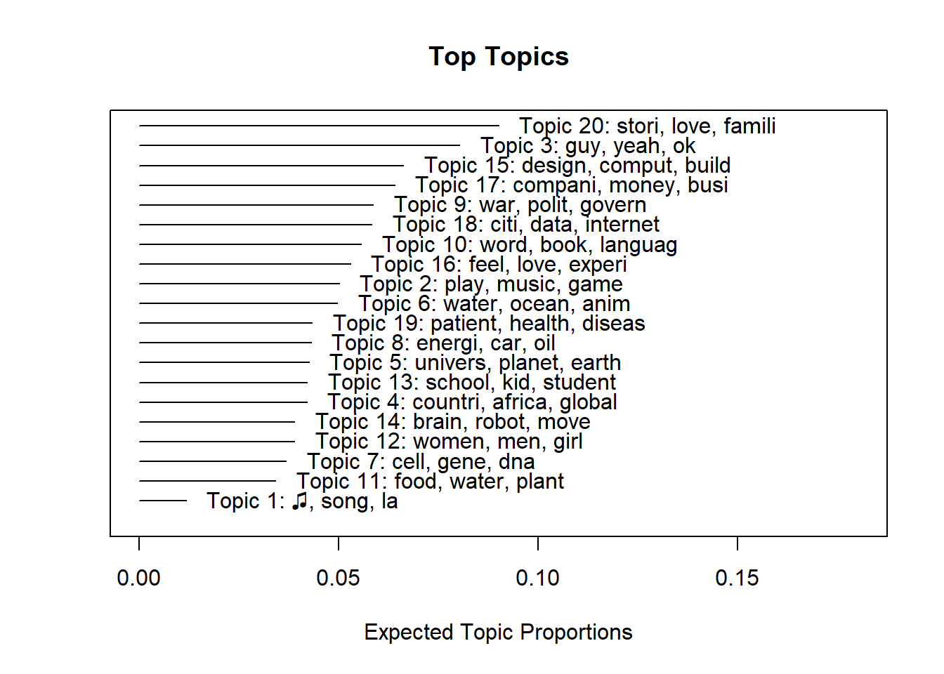
Or we could read about top words for all 20 topics (summary-function).
# By using summary() you receive top words for all 20 topics
summary(stm_20)
## A topic model with 20 topics, 2333 documents and a 4805 word dictionary.## Topic 1 Top Words:
## Highest Prob: <U+266B>, song, la, sing, oh, love, feel
## FREX: <U+266B>, la, song, sing, loop, oh, sheep
## Lift: <U+266B>, la, song, sing, coke, ski, ooh
## Score: <U+266B>, song, la, sing, music, ooh, feminist
## Topic 2 Top Words:
## Highest Prob: play, music, game, sound, art, film, artist
## FREX: artist, music, film, art, paint, game, play
## Lift: jersey, orchestra, cinema, opera, musician, music, masterpiec
## Score: jersey, music, art, film, paint, artist, game
## Topic 3 Top Words:
## Highest Prob: guy, yeah, ok, oh, stuff, sort, mayb
## FREX: guy, ok, yeah, stuff, oh, card, ca
## Lift: da, nerd, comedi, dude, yeah, guy, ok
## Score: da, ok, stuff, guy, ca, yeah, oh
## Topic 4 Top Words:
## Highest Prob: countri, africa, global, china, india, develop, state
## FREX: china, africa, india, chines, african, aid, countri
## Lift: curtain, ghana, capita, shanghai, sub-saharan, china, export
## Score: curtain, countri, africa, india, china, economi, chines
## Topic 5 Top Words:
## Highest Prob: univers, planet, earth, space, light, star, scienc
## FREX: galaxi, mar, particl, telescop, star, mathemat, orbit
## Lift: galaxi, hover, astronomi, spacecraft, telescop, asteroid, orbit
## Score: galaxi, telescop, particl, hover, mar, orbit, quantum
## Topic 6 Top Words:
## Highest Prob: water, ocean, anim, fish, tree, sea, forest
## FREX: ocean, forest, shark, sea, whale, coral, ice
## Lift: iceberg, reef, glacier, underwat, expedit, forest, canopi
## Score: iceberg, coral, ocean, forest, shark, speci, reef
## Topic 7 Top Words:
## Highest Prob: cell, gene, dna, bodi, biolog, organ, genet
## FREX: dna, gene, genom, cell, genet, tissu, molecul
## Lift: silk, chromosom, genom, dna, bacteri, mutat, tissu
## Score: silk, gene, cell, genom, dna, bacteria, tissu
## Topic 8 Top Words:
## Highest Prob: energi, car, oil, power, electr, percent, technolog
## FREX: oil, energi, car, fuel, nuclear, vehicl, electr
## Lift: fusion, emiss, coal, watt, brake, congest, renew
## Score: fusion, climat, co2, solar, carbon, energi, car
## Topic 9 Top Words:
## Highest Prob: war, polit, govern, state, power, law, countri
## FREX: prison, elect, vote, militari, crimin, polic, weapon
## Lift: toni, republican, terrorist, prosecut, bomber, crimin, diplomat
## Score: toni, democraci, islam, muslim, prison, polit, crimin
## Topic 10 Top Words:
## Highest Prob: word, book, languag, read, write, god, believ
## FREX: languag, religion, book, god, word, english, argument
## Lift: dictionari, meme, divin, bibl, linguist, verb, paragraph
## Score: dictionari, religion, languag, book, god, english, religi
## Topic 11 Top Words:
## Highest Prob: food, water, plant, eat, grow, farmer, product
## FREX: bee, food, farmer, mosquito, crop, vaccin, plant
## Lift: bee, mosquito, ebola, pesticid, crop, bread, flu
## Score: bee, food, mosquito, plant, vaccin, insect, farmer
## Topic 12 Top Words:
## Highest Prob: women, men, girl, woman, communiti, black, young
## FREX: women, men, gender, woman, girl, sex, gay
## Lift: grate, women, gender, feminist, gay, men, lesbian
## Score: grate, women, girl, men, gay, gender, woman
## Topic 13 Top Words:
## Highest Prob: school, kid, student, children, educ, teacher, teach
## FREX: school, teacher, kid, student, classroom, teach, educ
## Lift: pizza, tutor, classroom, curriculum, teacher, kindergarten, homework
## Score: pizza, school, teacher, kid, classroom, educ, student
## Topic 14 Top Words:
## Highest Prob: brain, robot, move, anim, neuron, bodi, control
## FREX: robot, neuron, brain, ant, monkey, conscious, memori
## Lift: ant, neuron, robot, lobe, neurosci, sensori, spinal
## Score: ant, robot, brain, neuron, cortex, neural, spinal
## Topic 15 Top Words:
## Highest Prob: design, comput, build, machin, technolog, project, sort
## FREX: design, comput, architectur, machin, 3d, fold, print
## Lift: fold, 3d, architectur, lego, pixel, printer, prototyp
## Score: fold, design, comput, architectur, 3d, build, machin
## Topic 16 Top Words:
## Highest Prob: feel, love, experi, happi, studi, social, emot
## FREX: compass, self, emot, psycholog, happi, moral, autism
## Lift: laughter, autism, happier, psychologist, self, disgust, adolesc
## Score: laughter, autism, social, compass, self, emot, sexual
## Topic 17 Top Words:
## Highest Prob: compani, money, busi, dollar, percent, market, product
## FREX: busi, compani, market, money, financi, dollar, innov
## Lift: calculus, investor, loan, mortgag, philanthropi, entrepreneuri, revenu
## Score: calculus, market, economi, money, econom, dollar, percent
## Topic 18 Top Words:
## Highest Prob: citi, data, internet, inform, network, build, connect
## FREX: internet, citi, network, onlin, web, twitter, facebook
## Lift: tedtalk, wikipedia, twitter, browser, upload, privaci, blogger
## Score: tedtalk, citi, data, twitter, inform, internet, web
## Topic 19 Top Words:
## Highest Prob: patient, health, diseas, cancer, medic, drug, doctor
## FREX: patient, medic, clinic, doctor, treatment, surgeri, hospit
## Lift: tom, physician, surgeri, medic, clinic, patient, cardiac
## Score: tom, patient, cancer, drug, diseas, health, medic
## Topic 20 Top Words:
## Highest Prob: stori, love, famili, walk, feel, home, man
## FREX: father, felt, son, knew, dad, walk, night
## Lift: mama, goodby, closet, grandfath, ash, homeless, fled
## Score: mama, father, famili, girl, dad, interview, love11.1.5 Validation and Model Selection
11.1.5.1 The optimal number of k
So far, we simply decided to set \(k\) (= the number of topics) to 20, i.e. we expect our collection of TED talks to be best represented with 20 topics. This was a simple guess. There are many different ways of how to specify \(k\) (informed guessing via theory and previous research, rule of thumb, manual labeling of a subset, statistical measures).
In the following we will focus on statistical measures, which is a comparatively fast and reasonable way of validating \(k\).
Steps:
- calculate multiple topic models with different specifications of k
- compare the models from Step 1 in terms of statistical measures
- based on Step 2, choose one specification of k
- eventually visualize and manually interpret your topic model of choice
We start with Step 1, which is calculating a larger number of topic models, each with a different specification of \(k\). Note, this might take a while, depending on your machine (for me 20 minutes).
# specify models with different k
stm_20_30_40_50 <- tibble(K = c(20, 30, 40, 50)) %>%
  mutate(model = map(K, ~ stm(out$documents,
                              out$vocab,
                              data=out$meta,
                              prevalence =  ~ s(date_num, degree = 2) +
                                dummy_female * dummy_white,
                              K = .,
                              verbose = FALSE)))
stm_20_30_40_50
#extract objects for single k values to perform regression and other analysis
stm20<-stm_20_30_40_50[[1,2]]
stm30<-stm_20_30_40_50[[2,2]]
stm40<-stm_20_30_40_50[[3,2]]
stm50<-stm_20_30_40_50[[4,2]]stm50## [[1]]
## A topic model with 50 topics, 2333 documents and a 4805 word dictionary.11.1.5.2 Semantic Coherence and Exclusivity
There are different statistical measures we can use to evaluate the models. Julia Silge here for instance introduces four: held-out likelihood, lower bound, residuals and semantic coherence. We will focus on the semantic coherence (a metric that correlates well with human judgment of topic quality) and additionally include exclusivity.
- Semantic coherence: how often do terms that have a high probability of belonging to one topic, also co-occur in the respective document? \(\rightarrow\) “the higher, the better”
- Exclusivity: How exclusive are the terms that occur with high probability for a topic; put differently: are they for other topics very unlikely? \(\rightarrow\) “the higher, the better”
We decide to not only consider semantic coherence (i.e., can easily be improved by simply modeling fewer topics -> larger vocabulary per topic) but to also consider exclusivity.
# calculate exclusivity + semantic coherence
model_scores <- stm_20_30_40_50 %>%
  mutate(exclusivity = map(model, exclusivity),
         semantic_coherence = map(model, semanticCoherence, out$documents)) %>%
  select(K, exclusivity, semantic_coherence)

model_scores #results in a nested dataframe containing the quantities of interest| K | exclusivity | semantic_coherence |
|---|---|---|
| 20 | 9.781185, 9.943524, 9.840624, 9.822129, 9.921995, 9.877850, 9.905818, 9.737277, 9.635212, 9.634374, 9.898207, 9.870780, 9.969914, 9.855582, 9.747229, 9.810443, 9.876303, 9.808596, 9.953805, 9.702340 | -48.36098, -62.87768, -39.29731, -38.51472, -79.33189, -60.95542, -60.15050, -59.17875, -59.42479, -38.11562, -93.22553, -47.84011, -50.85948, -67.49252, -45.86527, -54.47389, -49.50091, -47.78196, -47.08564, -43.20098 |
| 30 | 9.753890, 9.882566, 9.948838, 9.909858, 9.925477, 9.867925, 9.946908, 9.899083, 9.719962, 9.903003, 9.932988, 9.699905, 9.935665, 9.874112, 9.808498, 9.761734, 9.971818, 9.946623, 9.926611, 9.759464, 9.893159, 9.945018, 9.903886, 9.876799, 9.900915, 9.867815, 9.909494, 9.917283, 9.705940, 9.911053 | -47.28062, -78.24898, -45.48192, -55.32226, -57.28521, -67.29144, -62.86812, -65.91165, -65.54471, -59.60907, -68.10183, -54.10744, -58.76892, -72.48882, -44.34465, -52.66049, -50.65052, -61.07016, -66.25027, -37.94665, -72.96043, -71.85281, -71.51703, -46.71041, -55.65197, -80.90889, -51.24323, -55.88449, -38.70559, -67.99441 |
| 40 | 9.667174, 9.839923, 9.945988, 9.843621, 9.785777, 9.881130, 9.920281, 9.906531, 9.879427, 9.936875, 9.933679, 9.790257, 9.973418, 9.875428, 9.835685, 9.747966, 9.956840, 9.958625, 9.872589, 9.949177, 9.910855, 9.955425, 9.934096, 9.894234, 9.847775, 9.866756, 9.910274, 9.929505, 9.836213, 9.900754, 9.891181, 9.904500, 9.922682, 9.839310, 9.839723, 9.695839, 9.758461, 9.939982, 9.823852, 9.894570 | -37.81194, -57.30010, -49.50021, -56.10211, -51.42401, -84.66887, -57.59932, -62.14155, -58.61261, -58.66012, -70.69231, -56.37079, -69.69883, -72.24370, -50.08667, -61.59105, -49.59088, -75.16533, -69.85191, -44.78869, -70.52142, -44.16777, -72.00102, -91.67622, -48.90048, -67.41238, -47.53227, -59.22942, -50.76301, -70.60617, -81.15616, -59.18993, -75.72475, -47.87710, -95.25401, -39.44752, -59.26051, -63.16376, -55.63020, -49.62694 |
| 50 | 9.746418, 9.893381, 9.925573, 9.868023, 9.895456, 9.944297, 9.958534, 9.921006, 9.892510, 9.944077, 9.943115, 9.910005, 9.954565, 9.928538, 9.952929, 9.900940, 9.946806, 9.909799, 9.817226, 9.948099, 9.845306, 9.955109, 9.936018, 9.940261, 9.852087, 9.932254, 9.953523, 9.939317, 9.879848, 9.932469, 9.942733, 9.827533, 9.922415, 9.912235, 9.885159, 9.704620, 9.826186, 9.858001, 9.852816, 9.875649, 9.902083, 9.869540, 9.836237, 9.949089, 9.933785, 9.852031, 9.932659, 9.927430, 9.887911, 9.853624 | -44.82005, -82.89123, -60.76695, -51.32149, -72.75885, -87.27243, -55.58940, -59.29327, -69.12231, -63.21869, -69.62297, -70.71232, -60.03615, -73.33677, -79.91256, -87.44866, -49.49932, -71.21350, -81.40262, -45.20568, -57.04814, -78.81139, -71.98484, -45.94761, -37.40032, -88.53168, -66.67389, -62.70773, -54.35641, -59.40558, -69.81837, -60.21256, -74.64408, -56.80855, -108.38681, -43.07783, -51.93602, -79.41385, -66.67953, -48.45999, -51.41274, -67.65002, -89.18615, -84.35109, -86.28198, -64.96817, -74.73104, -79.78750, -73.83285, -69.93366 |
This data is best understood if we plot it. In my opinion most insights are generated by plotting semantic coherence and exclusivity against each other.
model_scores %>%
  select(K, exclusivity, semantic_coherence) %>%
  filter(K %in% c(20, 30, 50)) %>%
  unnest() %>%
  mutate(K = as.factor(K)) %>%
  ggplot(aes(semantic_coherence, exclusivity, color = K)) +
  geom_point(size = 2, alpha = 0.7) +
  labs(x = "Semantic coherence",
       y = "Exclusivity",
       title = "Comparing exclusivity and semantic coherence")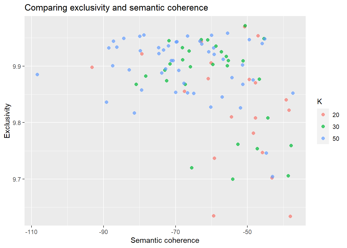
# upper right area indicates "good" topic model specifications# plot means for better overview
model_scores %>%
unnest(c(exclusivity, semantic_coherence)) %>%
group_by(K) %>%
summarize(exclusivity = mean(exclusivity),
semantic_coherence = mean(semantic_coherence)) %>%
ggplot(aes(x = semantic_coherence, y = exclusivity, color = as.factor(K))) +
geom_point() +
theme_bw()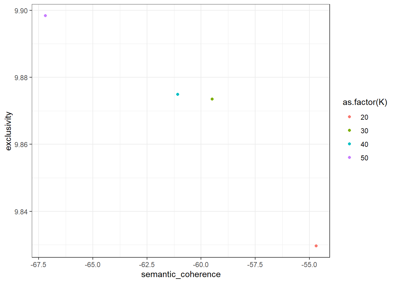
\(\rightarrow\) According to semantic coherence and exclusivity we should have a close look at TED Talks to be best represented by ~30 topics (in line with original findings from the paper)!
11.1.6 Visualization and Model Interpretation
Data visualization can help you in further analyzing your model of choice (k = 30). Let’s see what this topic model tells us about the Ted Talk Corpus and our research questions.
11.1.6.1 Word probabilities by topic
Here, we will look at the highest probability words per topic, which tells us more about the semantic meaning of a topic and is a common practice to find labels for the topics. For this we have to extract the \(ß\) (beta) values from our topic model, i.e., the probability of words belonging to topics which we can afterwards plot.
Most probably, for data visualization you will want to use ggplot2. To do so, we have to transform our stm30-object to a tidyverse compatible format using the tidytext-package.
td_beta <- tidy(stm30[[1]])

# Have a look; how is the word(stem) "absorb" displayed in this tidy dataframe?
td_beta[991:1020, 1:3]| topic | term | beta |
|---|---|---|
| 1 | absorb | 0.0000000 |
| 2 | absorb | 0.0000000 |
| 3 | absorb | 0.0000000 |
| 4 | absorb | 0.0000000 |
| 5 | absorb | 0.0003187 |
| 6 | absorb | 0.0000000 |
| 7 | absorb | 0.0005908 |
| 8 | absorb | 0.0006217 |
| 9 | absorb | 0.0000000 |
| 10 | absorb | 0.0000061 |
| 11 | absorb | 0.0001597 |
| 12 | absorb | 0.0000000 |
| 13 | absorb | 0.0000941 |
| 14 | absorb | 0.0002570 |
| 15 | absorb | 0.0000431 |
| 16 | absorb | 0.0000000 |
| 17 | absorb | 0.0000000 |
| 18 | absorb | 0.0000000 |
| 19 | absorb | 0.0000490 |
| 20 | absorb | 0.0000000 |
| 21 | absorb | 0.0000000 |
| 22 | absorb | 0.0000640 |
| 23 | absorb | 0.0004077 |
| 24 | absorb | 0.0000920 |
| 25 | absorb | 0.0000222 |
| 26 | absorb | 0.0000000 |
| 27 | absorb | 0.0000000 |
| 28 | absorb | 0.0001365 |
| 29 | absorb | 0.0001691 |
| 30 | absorb | 0.0000000 |
td_beta %>%
    group_by(topic) %>%
    top_n(4, beta) %>%
    ungroup() %>%
    mutate(topic = paste0("Topic ", topic),
           term = reorder_within(term, beta, topic)) %>%
    ggplot(aes(term, beta, fill = as.factor(topic))) +
    geom_col(alpha = 0.8, show.legend = FALSE) +
    facet_wrap(~ topic, scales = "free_y") +
    coord_flip() +
    scale_x_reordered() +
    labs(x = NULL, y = expression(beta),
         title = "Highest word probabilities for each topic",
         subtitle = "Different words are associated with different topics")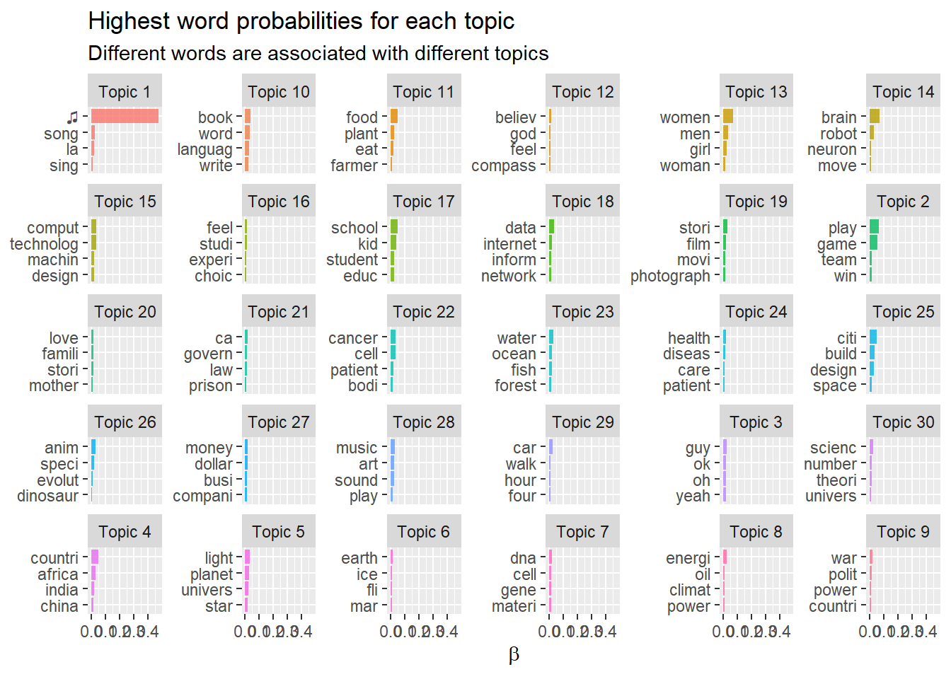
With an increasing number of topics and top words you want to display, text in this visualization becomes hard to read. If your interest is only in larger topics, consider the below plot (originally from Julia Silge).
td_gamma <- tidy(stm30[[1]], matrix = "gamma",
                 document_names = rownames(ted_dfm))

top_terms <- td_beta %>%
  arrange(beta) %>%
  group_by(topic) %>%
  top_n(7, beta) %>%
  arrange(-beta) %>%
  select(topic, term) %>%
  summarise(terms = list(term)) %>%
  mutate(terms = map(terms, paste, collapse = ", ")) %>%
  unnest()

gamma_terms <- td_gamma %>%
  group_by(topic) %>%
  summarise(gamma = mean(gamma)) %>%
  arrange(desc(gamma)) %>%
  left_join(top_terms, by = "topic") %>%
  mutate(topic = paste0("Topic ", topic),
         topic = reorder(topic, gamma))

gamma_terms %>%
  top_n(10, gamma) %>%
  ggplot(aes(topic, gamma, label = terms, fill = topic)) +
  geom_col(show.legend = FALSE) +
  geom_text(hjust = 0, nudge_y = 0.0005, size = 3) +
  coord_flip() +
  scale_y_continuous(expand = c(0,0),
                     limits = c(0, 0.09),
                     labels = percent_format()) +
  theme(plot.title = element_text(size = 16),
        plot.subtitle = element_text(size = 13)) +
  labs(x = NULL, y = expression(gamma),
       title = "Top topics by prevalence in the TED Talks corpus",
       subtitle = "With the top words that contribute to each topic")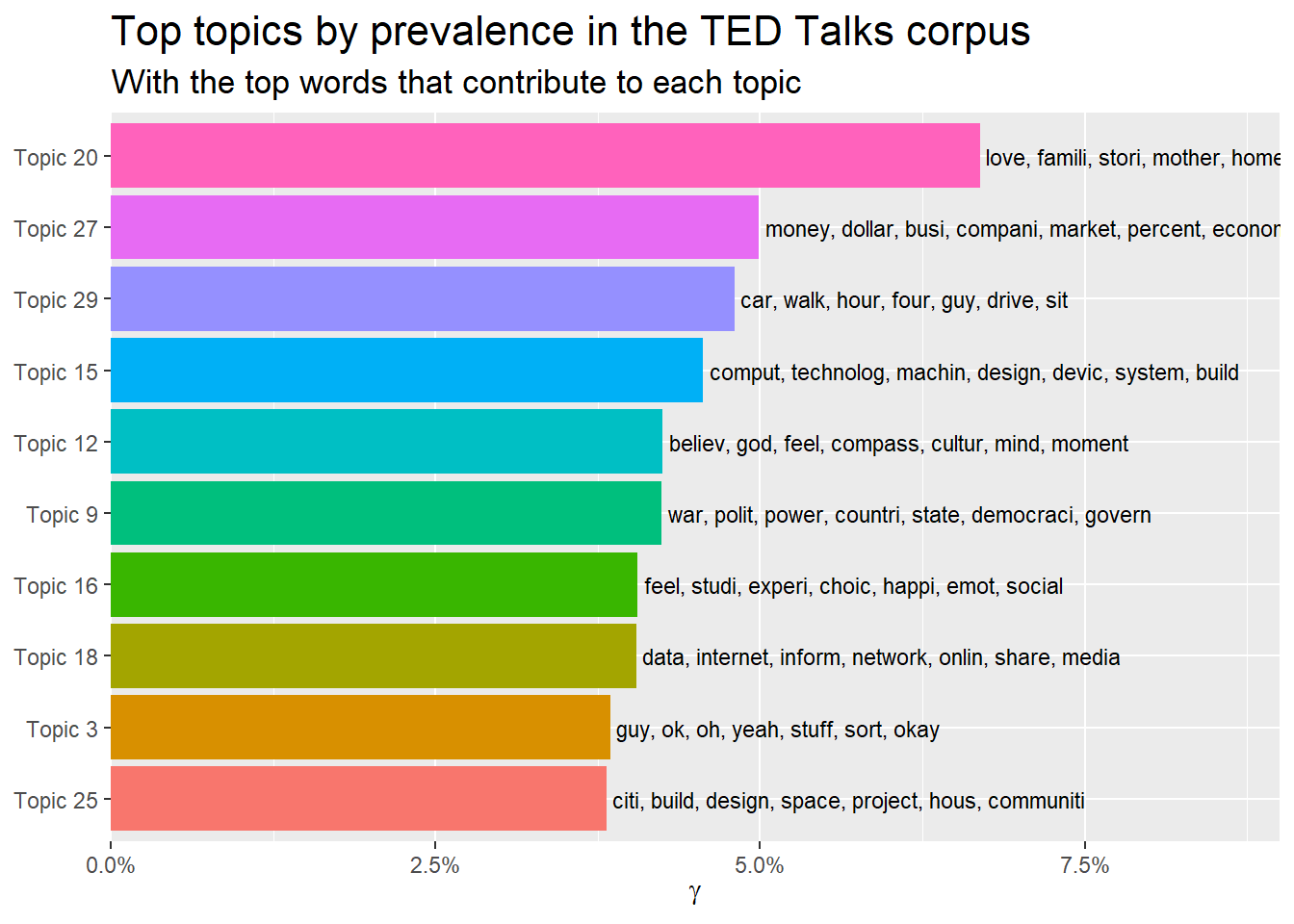
Also, you could of course stick to a tabular version (summary(stm30[[1]])). Also consider examining the FREX (frequency exclusivity) words which avoid prioritizing words that have high overall frequency but are not very exclusive to a topic.
summary(stm30[[1]])## A topic model with 30 topics, 2333 documents and a 4805 word dictionary.## Topic 1 Top Words:
## Highest Prob: <U+266B>, song, la, sing, love, oh, music
## FREX: <U+266B>, la, song, sing, loop, gonna, ooh
## Lift: <U+266B>, la, song, sing, coke, ooh, ski
## Score: <U+266B>, song, la, sing, ooh, poem, music
## Topic 2 Top Words:
## Highest Prob: play, game, team, win, player, video, feel
## FREX: game, player, win, toy, athlet, play, sport
## Lift: jersey, championship, game, athlet, basebal, player, olymp
## Score: game, jersey, play, player, coach, athlet, toy
## Topic 3 Top Words:
## Highest Prob: guy, ok, oh, yeah, stuff, sort, okay
## FREX: ok, yeah, oh, guy, okay, stuff, ted
## Lift: da, ok, yeah, oh, uh, um, dude
## Score: da, ok, yeah, oh, stuff, card, guy
## Topic 4 Top Words:
## Highest Prob: countri, africa, india, china, chines, african, state
## FREX: india, africa, china, african, chines, indian, villag
## Lift: curtain, ghana, india, nigeria, africa, african, china
## Score: curtain, africa, countri, india, china, african, chines
## Topic 5 Top Words:
## Highest Prob: light, planet, univers, star, earth, galaxi, dark
## FREX: galaxi, star, telescop, light, sun, dark, planet
## Lift: galaxi, hover, wavelength, astronomi, asteroid, telescop, jupit
## Score: galaxi, telescop, hover, planet, solar, asteroid, orbit
## Topic 6 Top Words:
## Highest Prob: earth, ice, fli, mar, feet, water, space
## FREX: ice, mar, pole, feet, cave, satellit, mountain
## Lift: iceberg, glacier, volcano, altitud, antarctica, ice, pole
## Score: iceberg, mar, ice, glacier, satellit, expedit, pole
## Topic 7 Top Words:
## Highest Prob: dna, cell, gene, materi, biolog, organ, molecul
## FREX: dna, genom, molecul, bacteria, gene, genet, sequenc
## Lift: silk, chromosom, genom, spider, microb, bacteria, mushroom
## Score: silk, bacteria, genom, gene, molecul, dna, microb
## Topic 8 Top Words:
## Highest Prob: energi, oil, climat, power, electr, percent, fuel
## FREX: oil, energi, fuel, nuclear, climat, electr, emiss
## Lift: fusion, coal, emiss, co2, watt, renew, fuel
## Score: fusion, climat, co2, carbon, solar, energi, emiss
## Topic 9 Top Words:
## Highest Prob: war, polit, power, countri, state, democraci, govern
## FREX: elect, democraci, vote, polit, muslim, militari, conflict
## Lift: toni, afghan, diplomat, republican, citizenship, bomber, civilian
## Score: toni, democraci, islam, muslim, polit, afghanistan, elect
## Topic 10 Top Words:
## Highest Prob: book, word, languag, write, read, english, speak
## FREX: languag, book, english, write, translat, cartoon, dictionari
## Lift: dictionari, spell, paragraph, cartoon, grammar, linguist, languag
## Score: dictionari, book, languag, poem, english, write, text
## Topic 11 Top Words:
## Highest Prob: food, plant, eat, farmer, farm, bee, grow
## FREX: food, bee, farmer, farm, crop, bread, agricultur
## Lift: bee, beef, chef, crop, bread, food, wheat
## Score: bee, food, plant, farmer, agricultur, crop, insect
## Topic 12 Top Words:
## Highest Prob: believ, god, feel, compass, cultur, mind, moment
## FREX: compass, self, religion, god, religi, faith, desir
## Lift: grate, compass, spiritu, medit, mystic, rabbi, self
## Score: grate, compass, religion, self, god, religi, spiritu
## Topic 13 Top Words:
## Highest Prob: women, men, girl, woman, black, young, sex
## FREX: women, men, gender, gay, girl, woman, sexual
## Lift: pizza, women, gay, gender, feminist, men, lesbian
## Score: women, pizza, men, girl, gay, gender, woman
## Topic 14 Top Words:
## Highest Prob: brain, robot, neuron, move, memori, bodi, control
## FREX: robot, neuron, brain, ant, memori, cortex, motor
## Lift: ant, robot, neuron, cortex, neurosci, neural, brain
## Score: ant, robot, brain, neuron, cortex, neural, spinal
## Topic 15 Top Words:
## Highest Prob: comput, technolog, machin, design, devic, system, build
## FREX: comput, machin, devic, technolog, fold, softwar, 3d
## Lift: fold, augment, 3d, comput, pixel, printer, machin
## Score: fold, comput, design, technolog, machin, algorithm, devic
## Topic 16 Top Words:
## Highest Prob: feel, studi, experi, choic, happi, emot, social
## FREX: choic, moral, psycholog, emot, relationship, bias, happi
## Lift: laughter, psychologist, disgust, psycholog, satisfact, happier, persuas
## Score: laughter, social, moral, emot, choic, psycholog, bias
## Topic 17 Top Words:
## Highest Prob: school, kid, student, educ, children, teacher, teach
## FREX: school, teacher, student, kid, educ, classroom, teach
## Lift: calculus, tutor, classroom, teacher, curriculum, kindergarten, grade
## Score: calculus, school, teacher, kid, educ, student, classroom
## Topic 18 Top Words:
## Highest Prob: data, internet, inform, network, onlin, share, media
## FREX: internet, onlin, data, twitter, web, googl, facebook
## Lift: tedtalk, twitter, blogger, browser, wikipedia, upload, facebook
## Score: tedtalk, data, twitter, internet, onlin, web, facebook
## Topic 19 Top Words:
## Highest Prob: stori, film, movi, photograph, imag, pictur, charact
## FREX: film, movi, photograph, charact, shot, tom, camera
## Lift: tom, filmmak, film, comedi, photographi, comic, cinema
## Score: tom, film, photograph, movi, storytel, comedi, camera
## Topic 20 Top Words:
## Highest Prob: love, famili, stori, mother, home, father, told
## FREX: father, mother, famili, mom, felt, sister, dad
## Lift: mama, goodby, uncl, father, birthday, hug, fled
## Score: mama, father, famili, mother, dad, love, mom
## Topic 21 Top Words:
## Highest Prob: ca, govern, law, prison, inform, secur, compani
## FREX: ca, prison, legal, crimin, patent, crime, polic
## Lift: ca, fraud, surveil, hacker, crimin, enforc, legal
## Score: ca, crimin, prison, hacker, surveil, polic, govern
## Topic 22 Top Words:
## Highest Prob: cancer, cell, patient, bodi, blood, diseas, heart
## FREX: cancer, surgeri, tumor, stem, breast, blood, surgeon
## Lift: devil, chemotherapi, tumor, cancer, surgeri, breast, surgic
## Score: devil, cancer, patient, tumor, cell, breast, tissu
## Topic 23 Top Words:
## Highest Prob: water, ocean, fish, forest, tree, sea, speci
## FREX: forest, whale, shark, fish, coral, ocean, reef
## Lift: whale, reef, forest, shark, coral, wildlif, dolphin
## Score: whale, coral, ocean, forest, shark, reef, fish
## Topic 24 Top Words:
## Highest Prob: health, diseas, care, patient, medic, drug, doctor
## FREX: health, vaccin, hiv, hospit, medic, diseas, infect
## Lift: alzheim, ebola, flu, vaccin, hiv, epidem, tuberculosi
## Score: alzheim, patient, diseas, health, hiv, vaccin, drug
## Topic 25 Top Words:
## Highest Prob: citi, build, design, space, project, hous, communiti
## FREX: citi, architectur, urban, architect, neighborhood, build, design
## Lift: lego, citi, architect, architectur, rio, urban, mayor
## Score: lego, citi, design, architectur, build, urban, architect
## Topic 26 Top Words:
## Highest Prob: anim, speci, evolut, dinosaur, natur, creatur, million
## FREX: dinosaur, chimpanze, evolut, monkey, extinct, ancestor, mosquito
## Lift: dinosaur, homo, chimpanze, sapien, ape, sperm, parasit
## Score: dinosaur, speci, chimpanze, mosquito, anim, mammal, insect
## Topic 27 Top Words:
## Highest Prob: money, dollar, busi, compani, market, percent, econom
## FREX: market, invest, capit, sector, busi, money, financi
## Lift: congest, investor, entrepreneuri, sector, philanthropi, entrepreneurship, profit
## Score: congest, economi, econom, market, sector, dollar, money
## Topic 28 Top Words:
## Highest Prob: music, art, sound, play, artist, paint, hear
## FREX: art, artist, music, paint, sound, musician, piano
## Lift: violin, orchestra, piano, musician, music, artist, artwork
## Score: violin, music, art, artist, paint, museum, sculptur
## Topic 29 Top Words:
## Highest Prob: car, walk, hour, four, guy, drive, sit
## FREX: car, morn, driver, seat, shoe, crash, drive
## Lift: jam, hobbi, pad, car, taxi, crash, candi
## Score: jam, car, driver, leg, lane, seat, ride
## Topic 30 Top Words:
## Highest Prob: scienc, number, theori, univers, model, mathemat, pattern
## FREX: theori, mathemat, particl, scienc, conscious, quantum, pattern
## Lift: symmetri, mathematician, quantum, mathemat, newton, theori, particl
## Score: symmetri, particl, quantum, mathemat, scienc, mathematician, theoriLast but not least, consider an interactive visualization, such as a shiny app to explore all your topics in a graphical way (great example here).