21.3 Lab: Classifier performance & fairness

See previous lab for notes.

library(tidyverse)
library(reshape2)
library(tidyverse)
set.seed(0)
# data <- read.csv("https://github.com/propublica/compas-analysis/raw/master/compas-scores-two-years.csv")
# write_csv(data, "compas-scores-two-years.csv")
data <- read_csv("compas-scores-two-years.csv")

See previous lab for notes.

# Add random vector
data <- data %>% mutate(random = sample(1:nrow(data)))
# Q: What happens here?

# First 5000 observations as training data
data_train <- data %>% filter(random >=1 & random<=5000)

# 1000 observations as test data
data_test <- data %>% filter(random >=5001 & random<=6000)

# 1000 observations as validation data
data.valid <- data %>% filter(random >=6001 & random<=7000)

See previous lab for notes.

fit <- glm(is_recid ~ age + priors_count, 
           family = binomial, 
           data = data_train)
#fit$coefficients
summary(fit)

## 
## Call:
## glm(formula = is_recid ~ age + priors_count, family = binomial, 
##     data = data_train)
## 
## Deviance Residuals: 
##     Min       1Q   Median       3Q      Max  
## -3.1159  -1.0670  -0.5752   1.1014   2.5503  
## 
## Coefficients:
##               Estimate Std. Error z value Pr(>|z|)    
## (Intercept)   1.014762   0.097015   10.46   <2e-16 ***
## age          -0.047415   0.002838  -16.71   <2e-16 ***
## priors_count  0.162316   0.008208   19.77   <2e-16 ***
## ---
## Signif. codes:  0 '***' 0.001 '**' 0.01 '*' 0.05 '.' 0.1 ' ' 1
## 
## (Dispersion parameter for binomial family taken to be 1)
## 
##     Null deviance: 6923.1  on 4999  degrees of freedom
## Residual deviance: 6200.0  on 4997  degrees of freedom
## AIC: 6206
## 
## Number of Fisher Scoring iterations: 4

21.3.1 Initial evaluation of the COMPAS scores

Here, we are computing the False Positive Rage (FPR), False Negative Rate (FNR) and the correct classification rate (CCR) for different populations.To do so we use the validation data data.valid. First, we’ll define functions to compute the quantities needed.

thr in the functions below is the threshold. is_recid incates whether someone recidivated.

# Function: False Positive Rate
get.FPR <- function(data.set, thr){
  return( # display results
    sum((data.set$decile_score >= thr) & 
    (data.set$is_recid == 0)) # Sum above threshold AND NOT recidivate
    /
    sum(data.set$is_recid == 0) # Sum NOT recividate
    )
}
# Share of people over the threshold that did not recidivate
# of all that did not recidivate (who got falsely predicted to
# recidivate)

# Q: Explain the function below!

# Function: False Negative Rate
get.FNR <- function(data.set, thr){
  return(sum((data.set$decile_score < thr) & 
               (data.set$is_recid == 1)) # ?
         /
           sum(data.set$is_recid == 1)) # ?
}

# Q: Explain the function below!
# Function: Correct Classification Rate
get.CCR <- function(data.set, thr){
  return(mean((data.set$decile_score >= thr) # ?
              == 
                data.set$is_recid)) # ?
}

Compute the data sets we need:

data.valid.b <- data.valid %>% filter(race == "African-American")
data.valid.w <- data.valid %>% filter(race == "Caucasian")

Now, we can compute the numbers:

thr <- 5

fps <- c(get.FPR(data.valid.b, 5), get.FPR(data.valid.w, 5), get.FPR(data.valid, 5))
fns <- c(get.FNR(data.valid.b, 5), get.FNR(data.valid.w, 5), get.FNR(data.valid, 5))
ccr <- c(get.CCR(data.valid.b, 5), get.CCR(data.valid.w, 5), get.CCR(data.valid, 5))

rates <- data.frame(FPR = fps, FNR = fns, CCR = ccr)
rownames(rates) = c("black", "white", "all")
rates

	FPR	FNR	CCR
black	0.4336283	0.2539062	0.6618257
white	0.2067308	0.4683544	0.6803279
all	0.2992278	0.3692946	0.6670000

We can see that the scores do not satisfy false positive parity and do not satisfy false negative parity. The scores do satisfy classification parity. Demographic parity is also not satisfied.

21.3.2 False positives negatives and correct classification

Let’s now obtain the FPR, FNR, and CCR for our own predictive logistic regression model, using the threshold \(0.5\). In the functions below we first generate predicted values for our outcome is_recid using the predict() function. Then we create a vector pred indicating whether those predicted values are above the threshold thr. Then we basically do the same as above, however, now we don’t use the COMPAS scores stored in decile_score but use our own predicted values. The predicted values are between 0 and 1 and not deciles as in decile_score. Hence, we have to change thr from 5 to 0.5.

# Functions to compute FPR, FNR, CCR using predicted values for 
# recidivism variable
get.FPR.fit <- function(thr, data.set, fit){
  pred <- predict(fit, newdata = data.set, type = "response") > thr
  return(sum((pred == 1) & (data.set$is_recid == 0))/sum(data.set$is_recid == 0))
}


get.FNR.fit <- function(thr, data.set, fit){
  pred <- predict(fit, newdata = data.set, type = "response") > thr
  return(sum((pred == 0) & (data.set$is_recid == 1))/sum(data.set$is_recid == 1))
}

get.CCR.fit <- function(thr, data.set, fit){
  pred <- predict(fit, newdata = data.set, type = "response") > thr
  return(mean(pred == data.set$is_recid))
}

# Create data subsets
data_train.b <- data_train %>% filter(race == "African-American")
data_train.w <- data_train %>% filter(race == "Caucasian")
data.valid.b <- data.valid %>% filter(race == "African-American")
data.valid.w <- data.valid %>% filter(race == "Caucasian")
thr <- .5 # define threshold

# Get results for training data
demo.perf.dat.train <- data.frame(FP =  c(get.FPR.fit(thr, data_train, fit),
                                          get.FPR.fit(thr, data_train.w, fit),
                                          get.FPR.fit(thr, data_train.b, fit)),
                                  FN =  c(get.FNR.fit(thr, data_train, fit),
                                          get.FNR.fit(thr, data_train.w, fit),
                                          get.FNR.fit(thr, data_train.b, fit)),
                                  CCR =  c(get.CCR.fit(thr, data_train, fit),
                                          get.CCR.fit(thr, data_train.w, fit),
                                          get.CCR.fit(thr, data_train.b, fit)))

demo.perf.dat.train

FP	FN	CCR
0.2736357	0.3757298	0.6774000
0.2068618	0.5289017	0.6607249
0.3604149	0.2777390	0.6853282

# Get results for validation data
demo.perf.dat.valid <- data.frame(FP =  c(get.FPR.fit(thr, data.valid, fit),
                                          get.FPR.fit(thr, data.valid.w, fit),
                                          get.FPR.fit(thr, data.valid.b, fit)),
                                  FN =  c(get.FNR.fit(thr, data.valid, fit),  
                                          get.FNR.fit(thr, data.valid.w, fit),
                                          get.FNR.fit(thr, data.valid.b, fit)),
                                  CCR =  c(get.CCR.fit(thr, data.valid, fit),
                                          get.CCR.fit(thr, data.valid.w, fit),
                                          get.CCR.fit(thr, data.valid.b, fit)))

demo.perf.dat.valid

FP	FN	CCR
0.2162162	0.3713693	0.7090000
0.1634615	0.4873418	0.6967213
0.3097345	0.2617188	0.7157676

It appears that there is basically no overfitting.

21.3.3 Altering the threshold

We can also explore how changing the threshold influences the false positive, false negative, and correct classification rates for the different groups (black, white, all). Below we write the function get.rates to get all the rates for a particular group for different threshold values. Then we write the plot.rates function to plot the rates for different groups.

# Get rates for different threshold values
# Function
get.rates <- function(thr, data.set){
  return(c(get.FPR(data.set, thr), get.FNR(data.set, thr), get.CCR(data.set, thr)))
}

# Execute function
thrs <- seq(0.5, 9.5, 1)
rates.w <- sapply(thrs, FUN=get.rates, data.valid.w)
rates.b <- sapply(thrs, FUN=get.rates, data.valid.b)
rates.all <- sapply(thrs, FUN=get.rates, data.valid)

# Function: plot rates
plot.rates <- function(thrs, rates, caption){
    rates.df <- data.frame(threshold = thrs, FPR = rates[1,], FNR = rates[2,], CCR = rates[3,])
    rates.df.tidy <- melt(rates.df, 1) %>% select(threshold = threshold, measure = variable, rate = value)
    ggplot(rates.df.tidy, mapping = aes(x = threshold, y = rate, color = measure)) +
      geom_smooth(se = F, method = "loess") + labs(title = caption)
}

We can now get three figures for the different demographics (let’s forego using facets again):

library(ggpubr)
p1 <- plot.rates(thrs, rates.w, "white defendants")
p2 <- plot.rates(thrs, rates.b, "black defendants")
p3 <- plot.rates(thrs, rates.all, "all defendants")
plots_combined <- ggarrange(p1, p2, p3,
  common.legend = TRUE,
  legend = "bottom",
  ncol = 3,
  nrow = 1
)
plots_combined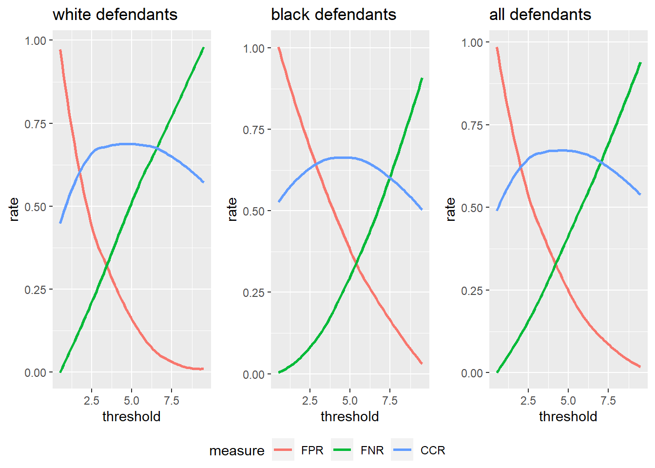 

21.3.4 Adjusting thresholds

We basically want to know how to we would need to adapt the thresholds for black and whites so that their false positive rates are at parity. In other words we would like to find the thresholds for which the false positive rates are at parity. Let’s see what the rates are for different thresholds.

thr <- c(0.3, 0.4, 0.51, 0.52, 0.53, 0.54, 0.55, 0.553, 0.555, 0.558, 0.56, 0.57, 0.58, 0.59, 0.7, 0.8)
fp.rates <- data.frame(thr = thr, 
                       FP.b  = sapply(thr, get.FPR.fit, data_train.b, fit),
                       FP.w = sapply(thr, get.FPR.fit, data_train.w, fit))

fp.rates

thr	FP.b	FP.w
0.300	0.8452895	0.6417760
0.400	0.6611927	0.4550959
0.510	0.3137424	0.1725530
0.520	0.2921348	0.1523713
0.530	0.2601556	0.1352170
0.540	0.2342264	0.1180626
0.550	0.2152118	0.1019173
0.553	0.2091616	0.0968718
0.555	0.2065687	0.0948537
0.558	0.1961971	0.0918264
0.560	0.1944685	0.0908174
0.570	0.1780467	0.0807265
0.580	0.1642178	0.0706357
0.590	0.1495246	0.0655903
0.700	0.0734659	0.0232089
0.800	0.0380294	0.0090817

We need to tweak the threshold for black defendants just a little:

plot.FPR <- function(fp.rates){
  colnames(fp.rates) <- c("thr", "African-American", "Caucasian")
  df.melted <- melt(fp.rates, "thr")
  colnames(df.melted) <- c("thr", "demographic", "FPR")
  ggplot(df.melted) + 
    geom_smooth(mapping=aes(x = thr, y = FPR, color = demographic), method = "loess", se = F) + 
    geom_vline(xintercept = 0.5, linetype = "dashed") + 
    geom_vline(xintercept = 0.553, linetype = "dashed") + 
    geom_hline(yintercept = 0.211, linetype = "dashed") + 
    ggtitle('FPR across thresholds')
}

plot.FPR(fp.rates)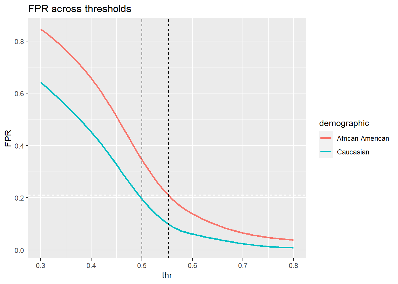

thr = 0.553 seems about right.

Now the white and black demographic would be at parity. We’ll compute the correct classification rate on the validation set.

n.correct <- sum(data_train.b$is_recid == (predict(fit, newdata = data_train.b, type = "response") > 0.553)) + 
             sum(data_train.w$is_recid == (predict(fit, newdata = data_train.w, type = "response") > 0.5))     
n.total <- nrow(data_train.b) + nrow(data_train.w)

n.correct/n.total

## [1] 0.6541072

(Note that we ignored everyone who wasn’t white or black. That’s OK to do, but including other demographics (in any way you like) is OK too).