13.1 Lab: Random Forest for text classification
The data comes from our project on measuring trust. The data for the lab was pre-processed. 56 open-ended answers that revealed the respondent’s profession, age, area of living/rown or others’ specific names/categories, particular activities (e.g., town elections) or city were deleted for reasons of anonymity.
We start by loading our data that contains the following variables:
id: Individual’s identification number (there is only one response per individual - so it’s also the id for the response)trust: Individual’s value on the trust scale- Question: Generally speaking, would you say that most people can betrusted, or that you can’t be too careful in dealing with people? Please tell me on a score of 0 to 6, where 0 means you can’t be too careful and 6 means that most people can be trusted.
- Original scale: 0 - You can’t be too careful; 1; 2; 3; 4; 5; 6 - Most people can be trusted; Don’t know;
- Recoded scale: Don’t know = NA and values 0-6 standardized to 0-1.
- Question: Generally speaking, would you say that most people can betrusted, or that you can’t be too careful in dealing with people? Please tell me on a score of 0 to 6, where 0 means you can’t be too careful and 6 means that most people can be trusted.
probing_answer: Individual’s response to the probing question- Question: In answering the previous question, who came to your mind when you were thinking about ‘most people?’ Please describe.
human_classified: Variable that contains the manual human classification of whether person was thinking about someone personally known to them or not (this is based on the open-ended response)- N = 295 were classified as 1 = yes
- N = 666 were classified as 0 = no
- N = 482 were not classified (we want to make predictions on those those!)
We start by loading the necessary packages and the data:
pacman::p_load(tidyverse, quanteda, tm, randomForest, varImp, ggwordcloud, kableExtra)
data <- read_csv("data/data_rf_lab.csv") %>%
  rename("trust_score" = "trust",
         "id_nr" = "id") %>% # rename variables (so that they don't mirror words in the dtm)
  mutate(training_data = !is.na(human_classified), # Add indicator for training data
         human_classified = as.factor(human_classified)) # Convert to factor so that randomForest() understands that it's classification
head(data) %>%
     kable("html") %>%
kable_styling(font_size = 9)| id_nr | trust_score | probing_answer | human_classified | training_data |
|---|---|---|---|---|
| 1 | 0.5000000 | People I know or have known a while. | NA | FALSE |
| 2 | 0.5000000 | Really everybody I know whether it be somebody I know as a neighbor or somebody I know as a friend somebody I know as a very close in a close relationship everybody has their limits of what they’re capable of doing and they may hit a wall and get to a point where they I feel threatened and acted in the erratic way but most people if I’m treating them with gentleness and respect we will have a decent interaction. But I just never know depends on how things are shaping up what kind of day everybody’s having. I suppose mostly I just have confidence in my ability to stay grounded in the flow of and Gestalt of interaction and find a current the river and float down the middle so to speak metaphorically. | 1 | TRUE |
| 3 | 0.6666667 | I thought about people I’ve met recently. One is a woman I met at the dog park I’ve become friends with | 1 | TRUE |
| 4 | 0.1666667 | Strangers and sometimes even work colleagues. | 1 | TRUE |
| 5 | 0.3333333 | I was clearly thinking of coworkers, 2 in particular where trust depended on whether or not there was something to gain by them being trustworthy or not. What they could get away with to their benefit | 1 | TRUE |
| 6 | 0.5000000 | Depends on the person. | NA | FALSE |
table(data$training_data)| FALSE | TRUE |
|---|---|
| 482 | 961 |
The variable human_classified contains the values NA (was not classified), 1 (respondents were thinking about people known to them) and 0 (respondents were not thinking about people known to them).
13.1.1 Preparing the data: DTM
Then we create a corpus and run some pre-processing functions (see discussion in previous sessions).
Q: What are we doing in the different steps below?
# cast text data into corpus
corpus <- Corpus(VectorSource(data$probing_answer)) %>%
  tm_map(removePunctuation, preserve_intra_word_dashes = TRUE) %>%  # ?
  tm_map(removeNumbers) %>% # ?
  tm_map(content_transformer(tolower)) %>%  # ?
  tm_map(removeWords, stopwords("english")) %>% # ?
  tm_map(stripWhitespace) %>%  # ?
  tm_map(stemDocument) # ?
Then we generate a DocumentTermMatrix (DTM) which we will use as a basis to train our ML model model_rf. Note that the matrix contains the frequency of various words in our open-ended responses.
# Create document term feature matrix
dtm <- DocumentTermMatrix(corpus) %>%
  removeSparseTerms(., 0.995) %>% # What are we doing here?
  as.matrix({.}) %>%
  as.data.frame({.})

# Add column names to matrix
colnames(dtm) = make.names(colnames(dtm)) # Make Syntactically Valid Names

# Illustration: Show subset of matrix
# show first, last columns
dtm %>%
  select(1:5, tail(names(.), 4)) %>%
  slice(1:8) %>%
  kable("html") %>%
kable_styling(font_size = 9)| know | known | peopl | close | day | anybodi | man | offic | seem |
|---|---|---|---|---|---|---|---|---|
| 1 | 1 | 1 | 0 | 0 | 0 | 0 | 0 | 0 |
| 5 | 0 | 1 | 2 | 1 | 0 | 0 | 0 | 0 |
| 0 | 0 | 1 | 0 | 0 | 0 | 0 | 0 | 0 |
| 0 | 0 | 0 | 0 | 0 | 0 | 0 | 0 | 0 |
| 0 | 0 | 0 | 0 | 0 | 0 | 0 | 0 | 0 |
| 0 | 0 | 0 | 0 | 0 | 0 | 0 | 0 | 0 |
| 0 | 0 | 2 | 0 | 0 | 0 | 0 | 0 | 0 |
| 0 | 0 | 0 | 0 | 0 | 0 | 0 | 0 | 0 |
Subsequently, we merge the DTM with our dataset (Just make sure you exclude the other variables that do not belong to the DTM when estimating the model later… see below…)
data <- bind_cols(data, dtm)

# Illustration: Show subset of data
# show first, last columns
data %>%
  select(1:5, tail(names(.), 4)) %>%
  slice(1:8) %>%
  kable("html") %>%
kable_styling(font_size = 9)| id_nr | trust_score | probing_answer | human_classified | training_data | anybodi | man | offic | seem |
|---|---|---|---|---|---|---|---|---|
| 1 | 0.5000000 | People I know or have known a while. | NA | FALSE | 0 | 0 | 0 | 0 |
| 2 | 0.5000000 | Really everybody I know whether it be somebody I know as a neighbor or somebody I know as a friend somebody I know as a very close in a close relationship everybody has their limits of what they’re capable of doing and they may hit a wall and get to a point where they I feel threatened and acted in the erratic way but most people if I’m treating them with gentleness and respect we will have a decent interaction. But I just never know depends on how things are shaping up what kind of day everybody’s having. I suppose mostly I just have confidence in my ability to stay grounded in the flow of and Gestalt of interaction and find a current the river and float down the middle so to speak metaphorically. | 1 | TRUE | 0 | 0 | 0 | 0 |
| 3 | 0.6666667 | I thought about people I’ve met recently. One is a woman I met at the dog park I’ve become friends with | 1 | TRUE | 0 | 0 | 0 | 0 |
| 4 | 0.1666667 | Strangers and sometimes even work colleagues. | 1 | TRUE | 0 | 0 | 0 | 0 |
| 5 | 0.3333333 | I was clearly thinking of coworkers, 2 in particular where trust depended on whether or not there was something to gain by them being trustworthy or not. What they could get away with to their benefit | 1 | TRUE | 0 | 0 | 0 | 0 |
| 6 | 0.5000000 | Depends on the person. | NA | FALSE | 0 | 0 | 0 | 0 |
| 7 | 0.8333333 | People I have interacted with during my life. Mainly people I have dealt with in my work experience. | NA | FALSE | 0 | 0 | 0 | 0 |
| 8 | 0.5000000 | 2 different types–the political and cultural extremists like anti-vaxxers and the majority in the middle | 0 | TRUE | 0 | 0 | 0 | 0 |
13.1.2 Training data & RF classifier training
To train our classifier we will only use the subset of the data (and dtm) for which we have labelled the outcome data in the variable human_classified, i.e., where human_classified is not NA (missing). To filter we can use our variable training_data that we generated above.
# Illustration: Show subset of data
# show first, last columns
data %>%
  filter(training_data) %>% # filters observations with TRUE
  select(1:5, tail(names(.), 3)) %>%
  slice(1:8) %>%
  kable("html") %>%
kable_styling(font_size = 9)| id_nr | trust_score | probing_answer | human_classified | training_data | man | offic | seem |
|---|---|---|---|---|---|---|---|
| 2 | 0.5000000 | Really everybody I know whether it be somebody I know as a neighbor or somebody I know as a friend somebody I know as a very close in a close relationship everybody has their limits of what they’re capable of doing and they may hit a wall and get to a point where they I feel threatened and acted in the erratic way but most people if I’m treating them with gentleness and respect we will have a decent interaction. But I just never know depends on how things are shaping up what kind of day everybody’s having. I suppose mostly I just have confidence in my ability to stay grounded in the flow of and Gestalt of interaction and find a current the river and float down the middle so to speak metaphorically. | 1 | TRUE | 0 | 0 | 0 |
| 3 | 0.6666667 | I thought about people I’ve met recently. One is a woman I met at the dog park I’ve become friends with | 1 | TRUE | 0 | 0 | 0 |
| 4 | 0.1666667 | Strangers and sometimes even work colleagues. | 1 | TRUE | 0 | 0 | 0 |
| 5 | 0.3333333 | I was clearly thinking of coworkers, 2 in particular where trust depended on whether or not there was something to gain by them being trustworthy or not. What they could get away with to their benefit | 1 | TRUE | 0 | 0 | 0 |
| 8 | 0.5000000 | 2 different types–the political and cultural extremists like anti-vaxxers and the majority in the middle | 0 | TRUE | 0 | 0 | 0 |
| 13 | 0.5000000 | The public in general, not my close friends | 0 | TRUE | 0 | 0 | 0 |
| 15 | 1.0000000 | Most of the people I know. Only a few are truly untrustworthy. However at first glance it is hard to tell. One of the managers at my last job came to mind. | 1 | TRUE | 0 | 0 | 0 |
| 16 | 0.3333333 | I first thought about strangers or unfamiliar people. I think my thought of “most people” mostly excluded close friends and family, who I feel can be trusted more than usual. | 0 | TRUE | 0 | 0 | 0 |
Based on the subset of the data that is labelled (training_data == TRUE) we can now train our classifier using the randomForest() function. Using human_classified ~ . below means that we use all the features, i.e., variables/columns in the DTM as predictors for human_classified (not that we excluded the id variable from the data). In our case, the features are dummies that indicate the presence of a particular word in the open-ended response. Importantly, since we attached the DTM to our dataset we have to exclude the relevant variable.
The randomForest() will build ntree trees to predict human_classified. ntree should be set sufficiently high “to ensure that every input row gets predicted at least a few times” (see ?randomForest()).
# Subset that is used below
head(data %>%
         filter(training_data) %>%
         select(-id_nr,
                -trust_score,
                -probing_answer,
-training_data))| human_classified | know | known | peopl | close | day | everybodi | feel | friend | get | interact | just | kind | may | middl | most | neighbor | never | realli | relationship | thing | way | ive | met | one | park | recent | thought | woman | colleagu | even | stranger | work | cowork | particular | someth | think | trust | trustworthi | person | experi | life | differ | like | major | alway | first | meet | nobodi | time | human | averag | general | might | public | see | store | street | year | popul | dont | came | hard | howev | job | mind | can | famili | usual | specif | citi | american | pictur | everyon | world | acquaint | complet | set | social | level | anyon | also | everyday | live | whole | back | place | someon | communiti | random | mean | neighborhood | societi | new | daili | deal | introduc | member | other | well | cant | encount | previous | circl | outsid | believ | lot | intent | past | say | want | around | seen | don.t | guy | across | come | relat | contact | age | race | errand | run | best | help | includ | busi | good | type | basi | imagin | larg | look | anyth | former | tri | hous | talk | pass | crowd | shop | co.work | regular | group | politician | make | worker | town | area | white | groceri | care | everi | answer | question | men | women | walk | school | etc | give | harm | guess | much | honest | ago | bad | situat | immedi | anybodi | man | offic | seem |
|---|---|---|---|---|---|---|---|---|---|---|---|---|---|---|---|---|---|---|---|---|---|---|---|---|---|---|---|---|---|---|---|---|---|---|---|---|---|---|---|---|---|---|---|---|---|---|---|---|---|---|---|---|---|---|---|---|---|---|---|---|---|---|---|---|---|---|---|---|---|---|---|---|---|---|---|---|---|---|---|---|---|---|---|---|---|---|---|---|---|---|---|---|---|---|---|---|---|---|---|---|---|---|---|---|---|---|---|---|---|---|---|---|---|---|---|---|---|---|---|---|---|---|---|---|---|---|---|---|---|---|---|---|---|---|---|---|---|---|---|---|---|---|---|---|---|---|---|---|---|---|---|---|---|---|---|---|---|---|---|---|---|---|---|---|---|---|---|---|---|---|---|---|
| 1 | 5 | 0 | 1 | 2 | 1 | 3 | 1 | 1 | 1 | 2 | 2 | 1 | 1 | 1 | 1 | 1 | 1 | 1 | 1 | 1 | 1 | 0 | 0 | 0 | 0 | 0 | 0 | 0 | 0 | 0 | 0 | 0 | 0 | 0 | 0 | 0 | 0 | 0 | 0 | 0 | 0 | 0 | 0 | 0 | 0 | 0 | 0 | 0 | 0 | 0 | 0 | 0 | 0 | 0 | 0 | 0 | 0 | 0 | 0 | 0 | 0 | 0 | 0 | 0 | 0 | 0 | 0 | 0 | 0 | 0 | 0 | 0 | 0 | 0 | 0 | 0 | 0 | 0 | 0 | 0 | 0 | 0 | 0 | 0 | 0 | 0 | 0 | 0 | 0 | 0 | 0 | 0 | 0 | 0 | 0 | 0 | 0 | 0 | 0 | 0 | 0 | 0 | 0 | 0 | 0 | 0 | 0 | 0 | 0 | 0 | 0 | 0 | 0 | 0 | 0 | 0 | 0 | 0 | 0 | 0 | 0 | 0 | 0 | 0 | 0 | 0 | 0 | 0 | 0 | 0 | 0 | 0 | 0 | 0 | 0 | 0 | 0 | 0 | 0 | 0 | 0 | 0 | 0 | 0 | 0 | 0 | 0 | 0 | 0 | 0 | 0 | 0 | 0 | 0 | 0 | 0 | 0 | 0 | 0 | 0 | 0 | 0 | 0 | 0 | 0 | 0 | 0 | 0 | 0 | 0 | 0 | 0 |
| 1 | 0 | 0 | 1 | 0 | 0 | 0 | 0 | 1 | 0 | 0 | 0 | 0 | 0 | 0 | 0 | 0 | 0 | 0 | 0 | 0 | 0 | 2 | 2 | 1 | 1 | 1 | 1 | 1 | 0 | 0 | 0 | 0 | 0 | 0 | 0 | 0 | 0 | 0 | 0 | 0 | 0 | 0 | 0 | 0 | 0 | 0 | 0 | 0 | 0 | 0 | 0 | 0 | 0 | 0 | 0 | 0 | 0 | 0 | 0 | 0 | 0 | 0 | 0 | 0 | 0 | 0 | 0 | 0 | 0 | 0 | 0 | 0 | 0 | 0 | 0 | 0 | 0 | 0 | 0 | 0 | 0 | 0 | 0 | 0 | 0 | 0 | 0 | 0 | 0 | 0 | 0 | 0 | 0 | 0 | 0 | 0 | 0 | 0 | 0 | 0 | 0 | 0 | 0 | 0 | 0 | 0 | 0 | 0 | 0 | 0 | 0 | 0 | 0 | 0 | 0 | 0 | 0 | 0 | 0 | 0 | 0 | 0 | 0 | 0 | 0 | 0 | 0 | 0 | 0 | 0 | 0 | 0 | 0 | 0 | 0 | 0 | 0 | 0 | 0 | 0 | 0 | 0 | 0 | 0 | 0 | 0 | 0 | 0 | 0 | 0 | 0 | 0 | 0 | 0 | 0 | 0 | 0 | 0 | 0 | 0 | 0 | 0 | 0 | 0 | 0 | 0 | 0 | 0 | 0 | 0 | 0 | 0 |
| 1 | 0 | 0 | 0 | 0 | 0 | 0 | 0 | 0 | 0 | 0 | 0 | 0 | 0 | 0 | 0 | 0 | 0 | 0 | 0 | 0 | 0 | 0 | 0 | 0 | 0 | 0 | 0 | 0 | 1 | 1 | 1 | 1 | 0 | 0 | 0 | 0 | 0 | 0 | 0 | 0 | 0 | 0 | 0 | 0 | 0 | 0 | 0 | 0 | 0 | 0 | 0 | 0 | 0 | 0 | 0 | 0 | 0 | 0 | 0 | 0 | 0 | 0 | 0 | 0 | 0 | 0 | 0 | 0 | 0 | 0 | 0 | 0 | 0 | 0 | 0 | 0 | 0 | 0 | 0 | 0 | 0 | 0 | 0 | 0 | 0 | 0 | 0 | 0 | 0 | 0 | 0 | 0 | 0 | 0 | 0 | 0 | 0 | 0 | 0 | 0 | 0 | 0 | 0 | 0 | 0 | 0 | 0 | 0 | 0 | 0 | 0 | 0 | 0 | 0 | 0 | 0 | 0 | 0 | 0 | 0 | 0 | 0 | 0 | 0 | 0 | 0 | 0 | 0 | 0 | 0 | 0 | 0 | 0 | 0 | 0 | 0 | 0 | 0 | 0 | 0 | 0 | 0 | 0 | 0 | 0 | 0 | 0 | 0 | 0 | 0 | 0 | 0 | 0 | 0 | 0 | 0 | 0 | 0 | 0 | 0 | 0 | 0 | 0 | 0 | 0 | 0 | 0 | 0 | 0 | 0 | 0 | 0 |
| 1 | 0 | 0 | 0 | 0 | 0 | 0 | 0 | 0 | 1 | 0 | 0 | 0 | 0 | 0 | 0 | 0 | 0 | 0 | 0 | 0 | 0 | 0 | 0 | 0 | 0 | 0 | 0 | 0 | 0 | 0 | 0 | 0 | 1 | 1 | 1 | 1 | 1 | 1 | 0 | 0 | 0 | 0 | 0 | 0 | 0 | 0 | 0 | 0 | 0 | 0 | 0 | 0 | 0 | 0 | 0 | 0 | 0 | 0 | 0 | 0 | 0 | 0 | 0 | 0 | 0 | 0 | 0 | 0 | 0 | 0 | 0 | 0 | 0 | 0 | 0 | 0 | 0 | 0 | 0 | 0 | 0 | 0 | 0 | 0 | 0 | 0 | 0 | 0 | 0 | 0 | 0 | 0 | 0 | 0 | 0 | 0 | 0 | 0 | 0 | 0 | 0 | 0 | 0 | 0 | 0 | 0 | 0 | 0 | 0 | 0 | 0 | 0 | 0 | 0 | 0 | 0 | 0 | 0 | 0 | 0 | 0 | 0 | 0 | 0 | 0 | 0 | 0 | 0 | 0 | 0 | 0 | 0 | 0 | 0 | 0 | 0 | 0 | 0 | 0 | 0 | 0 | 0 | 0 | 0 | 0 | 0 | 0 | 0 | 0 | 0 | 0 | 0 | 0 | 0 | 0 | 0 | 0 | 0 | 0 | 0 | 0 | 0 | 0 | 0 | 0 | 0 | 0 | 0 | 0 | 0 | 0 | 0 |
| 0 | 0 | 0 | 0 | 0 | 0 | 0 | 0 | 0 | 0 | 0 | 0 | 0 | 0 | 1 | 0 | 0 | 0 | 0 | 0 | 0 | 0 | 0 | 0 | 0 | 0 | 0 | 0 | 0 | 0 | 0 | 0 | 0 | 0 | 0 | 0 | 0 | 0 | 0 | 0 | 0 | 0 | 1 | 1 | 1 | 0 | 0 | 0 | 0 | 0 | 0 | 0 | 0 | 0 | 0 | 0 | 0 | 0 | 0 | 0 | 0 | 0 | 0 | 0 | 0 | 0 | 0 | 0 | 0 | 0 | 0 | 0 | 0 | 0 | 0 | 0 | 0 | 0 | 0 | 0 | 0 | 0 | 0 | 0 | 0 | 0 | 0 | 0 | 0 | 0 | 0 | 0 | 0 | 0 | 0 | 0 | 0 | 0 | 0 | 0 | 0 | 0 | 0 | 0 | 0 | 0 | 0 | 0 | 0 | 0 | 0 | 0 | 0 | 0 | 0 | 0 | 0 | 0 | 0 | 0 | 0 | 0 | 0 | 0 | 0 | 0 | 0 | 0 | 0 | 0 | 0 | 0 | 0 | 0 | 0 | 0 | 0 | 0 | 0 | 0 | 0 | 0 | 0 | 0 | 0 | 0 | 0 | 0 | 0 | 0 | 0 | 0 | 0 | 0 | 0 | 0 | 0 | 0 | 0 | 0 | 0 | 0 | 0 | 0 | 0 | 0 | 0 | 0 | 0 | 0 | 0 | 0 | 0 |
| 0 | 0 | 0 | 0 | 1 | 0 | 0 | 0 | 1 | 0 | 0 | 0 | 0 | 0 | 0 | 0 | 0 | 0 | 0 | 0 | 0 | 0 | 0 | 0 | 0 | 0 | 0 | 0 | 0 | 0 | 0 | 0 | 0 | 0 | 0 | 0 | 0 | 0 | 0 | 0 | 0 | 0 | 0 | 0 | 0 | 0 | 0 | 0 | 0 | 0 | 0 | 0 | 1 | 0 | 1 | 0 | 0 | 0 | 0 | 0 | 0 | 0 | 0 | 0 | 0 | 0 | 0 | 0 | 0 | 0 | 0 | 0 | 0 | 0 | 0 | 0 | 0 | 0 | 0 | 0 | 0 | 0 | 0 | 0 | 0 | 0 | 0 | 0 | 0 | 0 | 0 | 0 | 0 | 0 | 0 | 0 | 0 | 0 | 0 | 0 | 0 | 0 | 0 | 0 | 0 | 0 | 0 | 0 | 0 | 0 | 0 | 0 | 0 | 0 | 0 | 0 | 0 | 0 | 0 | 0 | 0 | 0 | 0 | 0 | 0 | 0 | 0 | 0 | 0 | 0 | 0 | 0 | 0 | 0 | 0 | 0 | 0 | 0 | 0 | 0 | 0 | 0 | 0 | 0 | 0 | 0 | 0 | 0 | 0 | 0 | 0 | 0 | 0 | 0 | 0 | 0 | 0 | 0 | 0 | 0 | 0 | 0 | 0 | 0 | 0 | 0 | 0 | 0 | 0 | 0 | 0 | 0 | 0 |
# train classifier based on labeled data and DTM
set.seed(100)
model_rf <- randomForest(human_classified ~ ., # "." = use all features
                                         data= data %>%
                                               filter(training_data) %>%
                                               select(-id_nr,
                                                      -trust_score,
                                                      -probing_answer,
                                                      -training_data),
                                         ntree=500) # number of trees

# By default, randomForest() consideres √p variables at each split when building a random forest of classification trees.
Just as for other model objects (results from estimations), the object of class randomForest has different components (see ?randomForest for the explanations we cite here). For instance, when we type model_rf$ntree we get the number of trees namely 500. Or model_rf$classes provides us with the classes of the outcome namely 0, 1.
We can also extract single trees from the random forest using the function getTree()
# See https://stats.stackexchange.com/a/461867
tree_model_rf <- randomForest::getTree(model_rf,
                                k = 1, # Take first tree
                                labelVar = TRUE) %>%
    tibble::rownames_to_column() %>%
    setNames(gsub(" ", "_", names(.))) %>% # replace blanks in varnames with underscore
    # make leaf split points to NA, so the 0s won't get plotted
    mutate(split_point = ifelse(is.na(prediction), split_point, NA))
head(tree_model_rf)| rowname | left_daughter | right_daughter | split_var | split_point | status | prediction |
|---|---|---|---|---|---|---|
| 1 | 2 | 3 | even | 0.5 | 1 | NA |
| 2 | 4 | 5 | friend | 0.5 | 1 | NA |
| 3 | 6 | 7 | stranger | 0.5 | 1 | NA |
| 4 | 8 | 9 | popul | 0.5 | 1 | NA |
| 5 | 10 | 11 | stranger | 1.5 | 1 | NA |
| 6 | 12 | 13 | honest | 0.5 | 1 | NA |
The resulting data frame describes the tree and contains various variables:
left_daughter: the row in the dataframetree_model_rfwhere the left daughter node is; 0 if the node is terminalright_daughter: the row in the dataframetree_model_rfwhere the right daughter node is; 0 if the node is terminal- split_var: which variable was used to split the node; 0 if the node is terminal
split_point: where the best split is; see Details for categorical predictorstatus: is the node terminal (-1) or not (1)prediction: the prediction for the node; 0 if the node is not terminal
In this particular tree the first split happened on the variable even and the cutoff was 0.5. The variable as the following values: Value: 0 (N = 950 ) Value: 1 (N = 11 ) and the corresponding observations are distributed between the two nodes.
Below – adapting some code from this example answer – we visualize the tree (you can also ignore the code as you won’t need it in your project). The graph does not show the full tree (only the first splits). It indicates on which variable the corresponding split occurred (e.g., even) and what the cutoff value was (e.g., 0.5). For a few branches we can already see the endnodes and the corresponding prediction (which corresponds to the mode/majority of oberverations in that node).
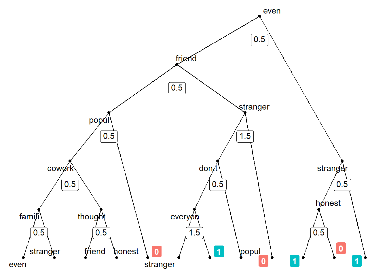
Let’s use the single tree to reiterate the logic of the random forest. Keep in mind that the steps below are repeated for each tree (here 500 times).
- Choose subset of the training set, i.e., sample of training observations.
- Take a random sample of \(m\) predictors as split candidates from the full set of \(p\) predictors. Default for classification is \(\sqrt{p}\). Here we have 172 predictors the square root of which is 13.114877. So we sample 13 predictors for each split.
- For the split the algorithm chooses the one predictor among those 13 that maximizes a certain criterion namely the Mean Decrease in Gini. Conceptually, it chooses the predictor/variables among the \(m\) predictors for which splitting leads to the highest level of node purity for the two daughter nodes. That is node purity in terms of our outcome variable thinking about strangers (0) or personally known other (1). A totally pure node would have only 0s or 1s in the node and a small Gini value would indicate that a node contains predominantly observations from a single class (cf. James et al. 2013, 312).
- Here predictor/variable even was used for the first split. Those observations that have a value below 0.5 end up in the left “daughter” node, the other ones in the right “daughter” node ( Left daugher (N = 950 ) Right daughter (N = 11 ) ).
- Steps 2. and 3. are repeated for each split.
- The algorithm stops splitting when the number of training samples in the node is less than a specified threshold. For classification the default is 1 (we can set this with the argument
nodesize =). - Important: There might be terminal nodes that have the same predicted value, i.e., a majority of the same values (either 0s or 1s). Such splits are sometimes conducted to increase node purity.
13.1.3 Evaluating the RF classifier
If we used randomForest() for classification, i.e., for classifying a categorical outcome, the component err.rate contains the “vector error rates of the prediction on the input data, the i-th element being the (OOB) error rate for all trees up to the i-th”. OOB here stands for out-of-bag. We can use that to obtain an estimate of the accuracy. See Out-of-Bag (OOB) Error Estimation for a quick overview (see ?randomForest and err.rate).
accuracy_content <- 1-mean(model_rf$err.rate[,1]) #82
accuracy_content
## [1] 0.8416143The component confusion contains the “confusion matrix of the prediction (based on OOB data)”. The rows represent the actual data, the columns the classifications from our ML model.
# confusion matrix of the prediction (based on OOB data)
model_rf$confusion| 0 | 1 | class.error | |
|---|---|---|---|
| 0 | 607 | 59 | 0.0885886 |
| 1 | 96 | 199 | 0.3254237 |
# rows: actual (what we want),
# columns: predicted
13.1.4 Exploring variable relevance & importance
And we discussed that different features/variables may play a more or less important role in our predictive model.
The function varUsed() can be used to show the features/variables that were actually used. If count=TRUE and by.tree=FALSE the result is an integer vector containing frequencies that variables are used in the forest in different trees. In total we have 172 feature resulting in the long vector below. For instance, the first number specifies the number of forests in which the first predictor has been used.
varUsed(model_rf) # Show frequencies of variable usage## [1] 1424 368 2496 691 461 316 172 1330 300 829 1287 216 504 44 188
## [16] 746 365 469 394 148 278 426 980 992 121 311 921 257 513 427
## [31] 1187 904 762 656 172 1335 1306 370 1170 266 787 353 711 479 279
## [46] 552 1165 516 588 303 704 1012 486 684 657 910 594 309 449 1029
## [61] 663 158 158 241 589 530 769 100 496 342 463 120 804 347 794
## [76] 145 174 266 139 850 228 447 580 63 151 212 563 545 773 339
## [91] 428 233 389 590 118 228 465 327 461 221 447 449 302 292 180
## [106] 332 144 426 214 156 446 157 150 101 130 443 480 191 186 171
## [121] 14 127 54 197 194 334 376 75 235 182 208 50 121 187 198
## [136] 278 231 103 261 250 622 311 489 244 72 283 235 287 189 232
## [151] 107 137 230 240 259 223 185 513 138 190 87 131 241 175 356
## [166] 322 101 269 293 513 308 20We could also visualize the usage frequency a wordcloud simply by joining the frequencies with the names of the features. Below we can see that peopl was one of the most used features used for tree splitting, albeit not necessarily the most important as we will see further below.
# Create dataset
data_plot <- data.frame(words = names(data %>%
         filter(training_data) %>%
         select(-id_nr,
                -trust_score,
                -probing_answer,
                -training_data,
                -human_classified))[1:length(varUsed(model_rf))],
                        frequency = varUsed(model_rf))

# Visualize
ggplot(data_plot, aes(label = words,
                      size = frequency,
                      color = frequency)) +
  geom_text_wordcloud_area() +
  theme_minimal() +
  scale_color_gradient(low = "darkred", high = "red")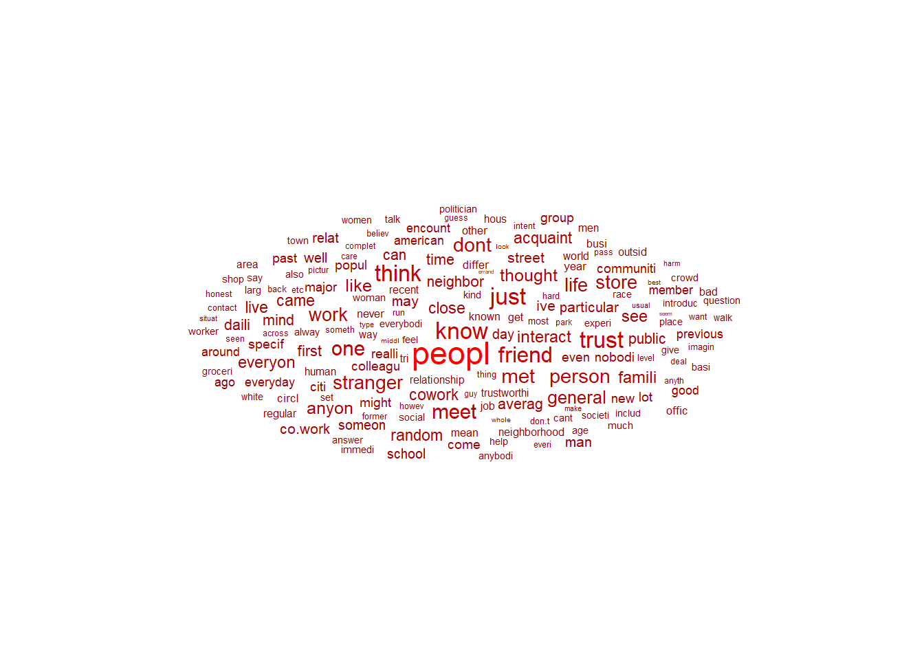
Finally, the importance() function can be used to extract the importance of different variables. For a quick explanation see Variable Importance Measures. The result makes sense. The variable friend indicating how often an open-ended response contained the word “friend” was the most features/variable for predicting whether the open-ended response was about personally known others or not.
# Plotting function from randomForest package
varImpPlot(model_rf)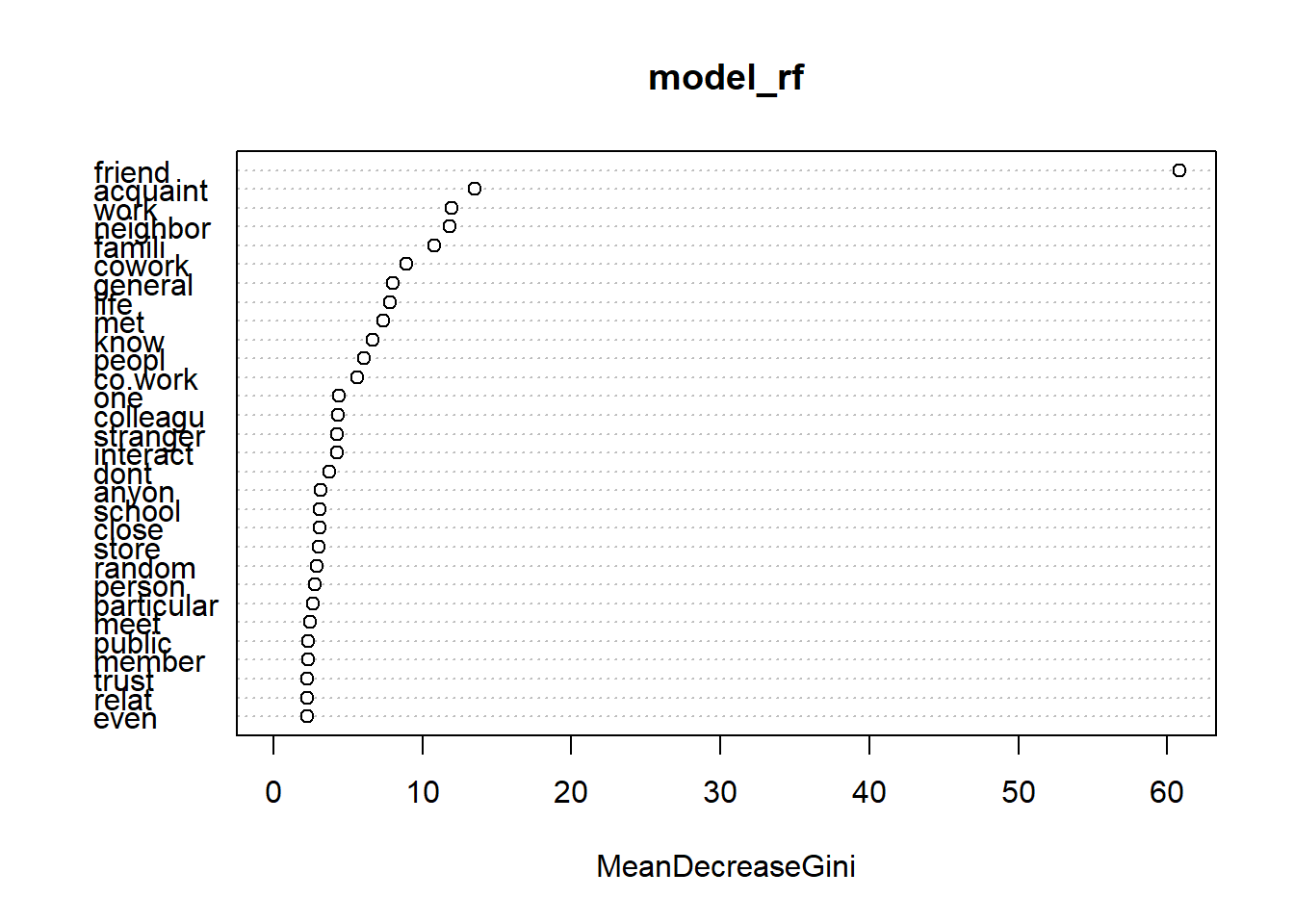
And below a nicer version of the same plot.
# Ggplot2 code
data_plot <- importance(model_rf) %>%
  data.frame() %>%
  mutate(variable = row.names(.)) %>%
  arrange(desc(MeanDecreaseGini)) %>%
  slice(1:20)

# Change to factor for ordering
data_plot$variable <- factor(data_plot$variable,
                             ordered = TRUE,
                             levels = rev(data_plot$variable))

  data_plot %>%
  ggplot(aes(x = MeanDecreaseGini, y = variable)) + # Change to +!
  geom_point() +
  ylab("Variable") +
  xlab("Importance: Mean Decrease of Gini") +
  theme_minimal()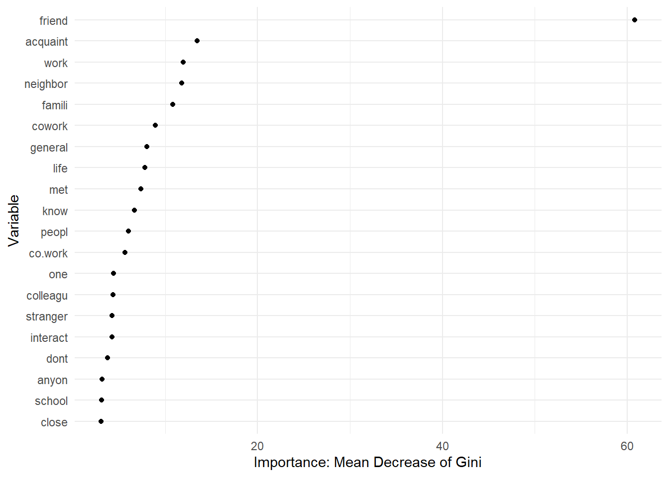
13.1.5 Add predictions to nonlabelled data
So far we have just explored our predictive model in the training dataset (the dataset for which we manually coded the outcome variable). But we haven’t used it to obtain predictions for observations where we don’t have outcome values, i.e., did not label the outcome variable. Below we use our random forest model to predict outcome values for the corresponding observations. We can extract the corresponding observations by filtering our dtm namely data %>% filter(!training_data) and specify this as newdata in the predict() function. Again we have to make sure that only the relevant variables are in there.
# DTM that contains only unlabeled documents, i.e. remove IDS from dtm that were part of test or training data
# Create dtm/dataset that only contains non-labelled observations
data_nonlabelled <- data %>% filter(!training_data)
nrow(data_nonlabelled)
## [1] 482# Add predictions as variable
data_nonlabelled$prediction <-
predict(model_rf, newdata = data_nonlabelled %>%
select(-id_nr, # Exclude relevant vars from prediction
-trust_score,
-probing_answer,
-training_data,
-human_classified))
# Illustration: Show subset of matrix
# show first, last columns
data_nonlabelled %>%
select(1:5, tail(names(.), 3)) %>%
slice(1:8) %>%
kable("html") %>%
kable_styling(font_size = 9)| id_nr | trust_score | probing_answer | human_classified | training_data | offic | seem | prediction |
|---|---|---|---|---|---|---|---|
| 1 | 0.5000000 | People I know or have known a while. | NA | FALSE | 0 | 0 | 1 |
| 6 | 0.5000000 | Depends on the person. | NA | FALSE | 0 | 0 | 0 |
| 7 | 0.8333333 | People I have interacted with during my life. Mainly people I have dealt with in my work experience. | NA | FALSE | 0 | 0 | 1 |
| 9 | 0.0000000 | Nobody in particular. I am always cautious with people I am meeting for the first time. | NA | FALSE | 0 | 0 | 0 |
| 10 | 0.0000000 | any and all humans | NA | FALSE | 0 | 0 | 0 |
| 11 | 0.5000000 | The general public, ie who I might see on the street or in a store on an average day. I tend to be trusting, but the last few years have made me less so after seeing more people in the express hateful views, intolerance, and only putting themselves first. | NA | FALSE | 0 | 0 | 0 |
| 12 | 0.5000000 | the general population | NA | FALSE | 0 | 0 | 0 |
| 14 | 0.3333333 | I was thinking of people I don’t know personally. | NA | FALSE | 0 | 0 | 0 |
13.1.6 Add predictions to labelled (training) data
We can also add predictions to our labelled (training) data. For that we first create an object data_labelled that contains the labelled observations (training_data = TRUE). The predictions may deviate from the actual outcome values that we find in the variable human_classified.
# Subset to get only labelled observations (training data)
data_labelled <- data %>%
            filter(training_data)

nrow(data_labelled)
## [1] 961# Predict values for labelled data using model
# Make sure to exclude vars "id" and "training_data"
data_labelled$prediction <- predict(model_rf,
data = data_labelled %>%
select(-id_nr, # Exclude relevant vars from prediction
-trust_score,
-probing_answer,
-training_data,
-human_classified))
# Illustration: Show subset of matrix
# show first, last columns
data_labelled %>%
select(1:5, tail(names(.), 3)) %>%
slice(1:8) %>%
kable("html") %>%
kable_styling(font_size = 9)| id_nr | trust_score | probing_answer | human_classified | training_data | offic | seem | prediction |
|---|---|---|---|---|---|---|---|
| 2 | 0.5000000 | Really everybody I know whether it be somebody I know as a neighbor or somebody I know as a friend somebody I know as a very close in a close relationship everybody has their limits of what they’re capable of doing and they may hit a wall and get to a point where they I feel threatened and acted in the erratic way but most people if I’m treating them with gentleness and respect we will have a decent interaction. But I just never know depends on how things are shaping up what kind of day everybody’s having. I suppose mostly I just have confidence in my ability to stay grounded in the flow of and Gestalt of interaction and find a current the river and float down the middle so to speak metaphorically. | 1 | TRUE | 0 | 0 | 1 |
| 3 | 0.6666667 | I thought about people I’ve met recently. One is a woman I met at the dog park I’ve become friends with | 1 | TRUE | 0 | 0 | 1 |
| 4 | 0.1666667 | Strangers and sometimes even work colleagues. | 1 | TRUE | 0 | 0 | 1 |
| 5 | 0.3333333 | I was clearly thinking of coworkers, 2 in particular where trust depended on whether or not there was something to gain by them being trustworthy or not. What they could get away with to their benefit | 1 | TRUE | 0 | 0 | 1 |
| 8 | 0.5000000 | 2 different types–the political and cultural extremists like anti-vaxxers and the majority in the middle | 0 | TRUE | 0 | 0 | 0 |
| 13 | 0.5000000 | The public in general, not my close friends | 0 | TRUE | 0 | 0 | 0 |
| 15 | 1.0000000 | Most of the people I know. Only a few are truly untrustworthy. However at first glance it is hard to tell. One of the managers at my last job came to mind. | 1 | TRUE | 0 | 0 | 0 |
| 16 | 0.3333333 | I first thought about strangers or unfamiliar people. I think my thought of “most people” mostly excluded close friends and family, who I feel can be trusted more than usual. | 0 | TRUE | 0 | 0 | 1 |
13.1.7 Creating the final dataset
Finally, we can simply bind the two datasubsets rowwise. data_final is the same as the original dataframe data only that it also contains our predictions in the variable prediction as well as the features/variables from the document-term-matrix.
data_final <- bind_rows(data_labelled,
                        data_nonlabelled )

# Illustration: Show subset of matrix
# show first, last columns
data_final %>%
    select(1:5, tail(names(.), 4)) %>%
    slice(1:8) %>%
  kable("html") %>%
kable_styling(font_size = 9)| id_nr | trust_score | probing_answer | human_classified | training_data | man | offic | seem | prediction |
|---|---|---|---|---|---|---|---|---|
| 2 | 0.5000000 | Really everybody I know whether it be somebody I know as a neighbor or somebody I know as a friend somebody I know as a very close in a close relationship everybody has their limits of what they’re capable of doing and they may hit a wall and get to a point where they I feel threatened and acted in the erratic way but most people if I’m treating them with gentleness and respect we will have a decent interaction. But I just never know depends on how things are shaping up what kind of day everybody’s having. I suppose mostly I just have confidence in my ability to stay grounded in the flow of and Gestalt of interaction and find a current the river and float down the middle so to speak metaphorically. | 1 | TRUE | 0 | 0 | 0 | 1 |
| 3 | 0.6666667 | I thought about people I’ve met recently. One is a woman I met at the dog park I’ve become friends with | 1 | TRUE | 0 | 0 | 0 | 1 |
| 4 | 0.1666667 | Strangers and sometimes even work colleagues. | 1 | TRUE | 0 | 0 | 0 | 1 |
| 5 | 0.3333333 | I was clearly thinking of coworkers, 2 in particular where trust depended on whether or not there was something to gain by them being trustworthy or not. What they could get away with to their benefit | 1 | TRUE | 0 | 0 | 0 | 1 |
| 8 | 0.5000000 | 2 different types–the political and cultural extremists like anti-vaxxers and the majority in the middle | 0 | TRUE | 0 | 0 | 0 | 0 |
| 13 | 0.5000000 | The public in general, not my close friends | 0 | TRUE | 0 | 0 | 0 | 0 |
| 15 | 1.0000000 | Most of the people I know. Only a few are truly untrustworthy. However at first glance it is hard to tell. One of the managers at my last job came to mind. | 1 | TRUE | 0 | 0 | 0 | 0 |
| 16 | 0.3333333 | I first thought about strangers or unfamiliar people. I think my thought of “most people” mostly excluded close friends and family, who I feel can be trusted more than usual. | 0 | TRUE | 0 | 0 | 0 | 1 |
In principle, we could also exclude the features/variables from the document-term-matrix again.
data_final <- data_final %>%
  select(id_nr, # Keep all relevant varst
         trust_score,
         probing_answer,
         training_data,
         human_classified,
         prediction)

# Illustration: Show subset of matrix
# show first, last columns
data_final %>%
    slice(1:8) %>%
  kable("html") %>%
kable_styling(font_size = 9)| id_nr | trust_score | probing_answer | training_data | human_classified | prediction |
|---|---|---|---|---|---|
| 2 | 0.5000000 | Really everybody I know whether it be somebody I know as a neighbor or somebody I know as a friend somebody I know as a very close in a close relationship everybody has their limits of what they’re capable of doing and they may hit a wall and get to a point where they I feel threatened and acted in the erratic way but most people if I’m treating them with gentleness and respect we will have a decent interaction. But I just never know depends on how things are shaping up what kind of day everybody’s having. I suppose mostly I just have confidence in my ability to stay grounded in the flow of and Gestalt of interaction and find a current the river and float down the middle so to speak metaphorically. | TRUE | 1 | 1 |
| 3 | 0.6666667 | I thought about people I’ve met recently. One is a woman I met at the dog park I’ve become friends with | TRUE | 1 | 1 |
| 4 | 0.1666667 | Strangers and sometimes even work colleagues. | TRUE | 1 | 1 |
| 5 | 0.3333333 | I was clearly thinking of coworkers, 2 in particular where trust depended on whether or not there was something to gain by them being trustworthy or not. What they could get away with to their benefit | TRUE | 1 | 1 |
| 8 | 0.5000000 | 2 different types–the political and cultural extremists like anti-vaxxers and the majority in the middle | TRUE | 0 | 0 |
| 13 | 0.5000000 | The public in general, not my close friends | TRUE | 0 | 0 |
| 15 | 1.0000000 | Most of the people I know. Only a few are truly untrustworthy. However at first glance it is hard to tell. One of the managers at my last job came to mind. | TRUE | 1 | 0 |
| 16 | 0.3333333 | I first thought about strangers or unfamiliar people. I think my thought of “most people” mostly excluded close friends and family, who I feel can be trusted more than usual. | TRUE | 0 | 1 |
13.1.8 How to create a training dataset
First, we would load the full dataset that contains the texts. Below we have a dataset with tweets that we classify.
data <- read_csv("data/data_tweets_de.csv",
                 col_types = cols(.default = "c")) %>% # Make sure to read in columns as character (otherwise you will get problem with long numbers)
  select(text, retweet_count, id_str, user_id_str) %>%
  slice(1:1000) %>% # Take the first 1000 observations as an example
  mutate(id_nr = row_number())
set.seed(100)
data <- data %>% sample_n(size = nrow(.)) # Randomly reorder rows
# Why would we randomly reorder rows?
Then we store the data locally in an excel file. Make sure that any data you export or import always contains a unique classifier (we created one above called id_nr).
write_excel_csv(data, "data/data_for_coding.csv")We open the excel file and save it under another name, e.g., data_for_coding_paul.csv if the person who codes the sample is called Paul.
In this new excel file we create a variable called human_classified (or any other name) and label as many observations as possible following our coding scheme.
Then we import the data file the contains the labelled outcome stored in human_classified.
data <- read_csv("data/data_for_coding_paul.csv")Then we create a variable training_data that indicates which observations have been labelled.
data <- data %>%
  mutate(training_data = !is.na(human_classified))
And we can check how many we have classified (here I classified only few observations).
table(data$training_data)| FALSE | TRUE |
|---|---|
| 982 | 18 |
After that we would basically proceed as described in the lab above. If you don’t want to export the full dataset for manual labelling chose a subset and join the datasets again later (just make sure you have a unique identifer for joining).
Besides, it may make sense to label with two persons and discuss tricky cases and code them together.