10.3 (R-)Workflow for Text Analysis
Data collection (“Obtaining Text”*)
Data manipulation / Corpus pre-processing (“From Text to Data”*)
Vectorization: Turning Text into a Matrix (DTM/DFM) (“From Text to Data”*)
Analysis (“Quantitative Analysis of Text”*)
Validation and Model Selection (“Evaluating Performance”*) (lab only)
Visualization and Model Interpretation (lab only)
10.3.1 Data collection
- use existing corpora
- collect new corpora
- electronic sources (Application user interfaces (APIs), Web Scraping), e.g. twitter, wikipedia, transcripts of all german electoral programs
- undigitized text, e.g. scans of documents
- data from interviews, surveys and/or experiments
- consider relevant applications to turn your data into text format (speech-to-text recognition, pdf-to-text, OCR, Mechanical Turk and Crowdflower)
10.3.2 Data manipulation: Basics (1)
- text data is different from “structured” data (e.g., a set of rows and columns)
- most often not “clean” but rather messy
- shortcuts, dialect, incorrect grammar, missing words, spelling issues, ambiguous language, humor
- web context: emojis, # (twitter), etc.
- Investing some time in carefully cleaning and preparing your data might be one of the most crucial determinants for a successful text analysis!
10.3.3 Data manipulation: Basics (2)
Common steps in pre-processing text data:
- stemming (removal of word suffixes), e.g., computation, computational, computer \(\rightarrow\) compute; or lemmatisation (reduce a term to its lemma, i.e., its base form), e.g., “better” \(\rightarrow\) “good”
- transformation to lower cases
- removal of punctuation (e.g., ,;.-) / numbers / white spaces / URLs / stopwords / very infrequent words
\(\rightarrow\) Always choose your prepping steps carefully! Removing punctuation for instance might be a good idea in many projects, however think of unfortunate cases: “I enjoy: eating, my cat and leaving out commas” vs. “I enjoy: eating my cat and leaving out commas” + unit of analysis! (sentence vs. unigram)
10.3.4 Data manipulation: Basics (3)
In principle, all those transformations can be achieved by using base R
Other packages however provide ready-to-apply functions, such as {tidytext}, {tm} or {quanteda}
Important: to start pre-processing with these packages your data always has to be first transformed to a corpus object or alternatively to a tidy text object (examples on the next slides)
10.3.5 Data manipulation: Tidytext Example (1)
Pre-processing with tidytext requires your data to be stored in a tidy text object.
Q: What are main characteristics of a tidy text dataset?
- one-token-per-row
- “long format”
First, we have to retrieve some data. In keeping with today’s session, we will use data from Wikipedias entry on Natural Language Processing.
# load and install packages if neccessary
if(!require("rvest")) {install.packages("rvest"); library("rvest")}
if(!require("xml2")) {install.packages("xml2"); library("xml2")}
if(!require("tidytext")) {install.packages("tidytext"); library("tidytext")}
if(!require("tibble")) {install.packages("tibble"); library("tibble")}
if(!require("dplyr")) {install.packages("dplyr"); library("dplyr")}
# import wikipedia entry on Natural Language Processing, parsed by paragraph
text <- read_html("https://en.wikipedia.org/wiki/Natural_language_processing#Text_and_speech_processing") %>%
html_nodes("#content p")%>%
html_text()
# we decide to keep only paragraph 1 and 2
text<-text[1:2]
text## [1] "Natural language processing (NLP) is a subfield of linguistics, computer science, and artificial intelligence concerned with the interactions between computers and human language, in particular how to program computers to process and analyze large amounts of natural language data. The goal is a computer capable of \"understanding\" the contents of documents, including the contextual nuances of the language within them. The technology can then accurately extract information and insights contained in the documents as well as categorize and organize the documents themselves.\n"
## [2] "Challenges in natural language processing frequently involve speech recognition, natural-language understanding, and natural-language generation.\n"In order to turn this data into a tidy text dataset, we first need to put it into a data frame (or tibble).
# put character vector into a data frame
# also add information that data comes from the wiki entry on NLP and from which paragraphs
wiki_df <- tibble(topic=c("NLP"), paragraph=1:2, text=text)

str(wiki_df)
## tibble [2 x 3] (S3: tbl_df/tbl/data.frame)
## $ topic : chr [1:2] "NLP" "NLP"
## $ paragraph: int [1:2] 1 2
## $ text : chr [1:2] "Natural language processing (NLP) is a subfield of linguistics, computer science, and artificial intelligence c"| __truncated__ "Challenges in natural language processing frequently involve speech recognition, natural-language understanding"| __truncated__Q: Describe the above dataset. How many variables and observations are there? What do the variables display?
Now, by using the unnest_tokens() function from tidytext we transform this data to a tidy text format.
# Create tidy text format and remove stopwords
tidy_df <- wiki_df %>%
  unnest_tokens(word, text) %>%
  anti_join(stop_words)
Q: How does our dataset change after tokenization and removing stopwords? How many observations do we now have? And what does the paragraph variable identify/store?
Q: Also, have a closer look at the single words. Do you notice anything else that has changed, e.g., is something missing from the original text?
str(tidy_df,10)## tibble [57 x 3] (S3: tbl_df/tbl/data.frame)
## $ topic : chr [1:57] "NLP" "NLP" "NLP" "NLP" ...
## $ paragraph: int [1:57] 1 1 1 1 1 1 1 1 1 1 ...
## $ word : chr [1:57] "natural" "language" "processing" "nlp" ...tidy_df$word[1:15]## [1] "natural" "language" "processing" "nlp" "subfield"
## [6] "linguistics" "computer" "science" "artificial" "intelligence"
## [11] "concerned" "interactions" "computers" "human" "language"10.3.6 Data manipulation: Tidytext Example (2)
“Pros” and “Cons”:
tidytext removes punctuation and makes all terms lowercase automatically (see above)
all other transformations need some dealing with regular expressions
- example to remove white space with tidytext (s+ describes a blank space):
example_white_space <- gsub("\\s+","",wiki_df$text)
example_white_space
## [1] "Naturallanguageprocessing(NLP)isasubfieldoflinguistics,computerscience,andartificialintelligenceconcernedwiththeinteractionsbetweencomputersandhumanlanguage,inparticularhowtoprogramcomputerstoprocessandanalyzelargeamountsofnaturallanguagedata.Thegoalisacomputercapableof\"understanding\"thecontentsofdocuments,includingthecontextualnuancesofthelanguagewithinthem.Thetechnologycanthenaccuratelyextractinformationandinsightscontainedinthedocumentsaswellascategorizeandorganizethedocumentsthemselves."
## [2] "Challengesinnaturallanguageprocessingfrequentlyinvolvespeechrecognition,natural-languageunderstanding,andnatural-languagegeneration."- \(\rightarrow\) consider alternative packages (e.g., tm, quanteda)
Example: tm package
- input: corpus not tidytext object
- What is a corpus in R? \(\rightarrow\) group of documents with associated metadata
# Load the tm package
library(tm)

# Clean corpus
corpus_clean <- VCorpus(VectorSource(wiki_df$text)) %>%
  tm_map(removePunctuation, preserve_intra_word_dashes = TRUE) %>%
  tm_map(removeNumbers) %>%
  tm_map(content_transformer(tolower)) %>%
  tm_map(removeWords, words = c(stopwords("en"))) %>%
  tm_map(stripWhitespace) %>%
  tm_map(stemDocument)

# Check exemplary document
corpus_clean[["1"]][["content"]]
## [1] "natur languag process nlp subfield linguist comput scienc artifici intellig concern interact comput human languag particular program comput process analyz larg amount natur languag data goal comput capabl understand content document includ contextu nuanc languag within technolog can accur extract inform insight contain document well categor organ document"- with the tidy text format, regular R functions can be used instead of the specialized functions which are necessary to analyze a corpus object
- dplyr workflow to count the most popular words in your text data:
tidy_df %>% count(word) %>% arrange(desc(n))- especially for starters, tidytext is a good starting point (in my opinion), since many steps has to be carried out individually (downside: maybe more code)
- other packages combine many steps into one single function (e.g. quanteda combines pre-processing and DFM casting in one step)
- R (as usual) offers many ways to achieve similar or same results
- e.g. you could also import, filter and pre-process using dplyr and tidytext, further pre-process and vectorize with tm or quanteda (tm has simpler grammar but slightly fewer features), use machine learning applications and eventually re-convert to tidy format for interpretation and visualization (ggplot2)
10.3.7 Vectorization: Basics
- Text analytical models (e.g., topic models) often require the input data to be stored in a certain format
- only so will algorithms be able to quickly compare one document to a lot of other documents to identify patterns
- Typically: document-term matrix (DTM), sometimes also called document-feature matrix (DFM)
- turn raw text into a vector-space representation
- matrix where each row represents a document and each column represents a word
- term-frequency (tf): the number within each cell describes the number of times the word appears in the document
- term frequency–inverse document frequency (tf-idf): weights the occurrence of certain words, e.g., lowering the weight of the word “education” in an corpus of articles on educational inequality
10.3.8 Vectorization: Tidytext example
Remember our tidy text formatted data (“one-token-per-row”)?
print(tidy_df[1:5,])## # A tibble: 5 x 3
## topic paragraph word
## <chr> <int> <chr>
## 1 NLP 1 natural
## 2 NLP 1 language
## 3 NLP 1 processing
## 4 NLP 1 nlp
## 5 NLP 1 subfieldWith the cast_dtm function from the tidytext package, we can now transform it to a DTM.
# Cast tidy text data into DTM format
dtm <- tidy_df %>%
  count(paragraph,word) %>%
  cast_dtm(document=paragraph,
                 term=word,
                 value=n) %>%
        as.matrix()

# Check the dimensions and a subset of the DTM
dim(dtm)
## [1] 2 41print(dtm[,1:6]) # important: this is only a snippet of the DTM (6 terms only)## Terms
## Docs accurately amounts analyze artificial capable categorize
## 1 1 1 1 1 1 1
## 2 0 0 0 0 0 010.3.9 Vectorization: Tm example
- In case you pre-processed your data with the tm package, remember we ended with a pre-processed corpus object
- Now, simply apply the DocumentTermMatrix function to this corpus object
# Pass your "clean" corpus object to the DocumentTermMatrix function
dtm_tm <- DocumentTermMatrix(corpus_clean, control = list(wordLengths = c(2, Inf))) # control argument here is specified to include words that are at least two characters long

# Check a subset of the DTM
inspect(dtm_tm[,1:6])
## <<DocumentTermMatrix (documents: 2, terms: 6)>>
## Non-/sparse entries: 6/6
## Sparsity : 50%
## Maximal term length: 8
## Weighting : term frequency (tf)
## Sample :
## Terms
## Docs accur amount analyz artifici can capabl
## 1 1 1 1 1 1 1
## 2 0 0 0 0 0 0Q: How do the terms between the DTM we created with tidytext and the one created with tm differ? Why?
10.3.10 Analysis: Supervised vs. unsupervised
- Supervised statistical learning: involves building a statistical model for predicting, or estimating, an output based on one or more inputs
- We observe both features \(x_{i}\) and the outcome \(y_{i}\)
- Unsupervised statistical learning: There are inputs but no supervising output; we can still learn about relationships and structure from such data
- choice might depend on specific use case: “Whereas unsupervised methods are often used for discovery, supervised learning methods are primarily used as a labor-saving device.” (Wilkerson and Casas 2017)
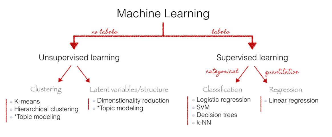
Source: Christine Doig 2015, also see Grimmer and Stewart (2013) for an overview of text as data methods.
10.3.11 Topic Modeling
- Goal: discovering the hidden (i.e, latent) topics within the documents and assigning each of the topics to the documents
- topic models belong to a class of unsupervised classification
- i.e., no prior knowledge of a corpus’ content or its inherent topics is needed (however some knowledge might help you validate your model later on)
- Researcher only needs to specify number of topics (not as intuitive as it sounds!)
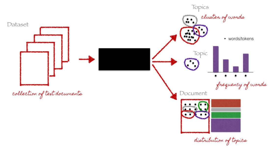
Source: Christine Doig 2015
10.3.12 Topic Modeling: Latent Dirichlet Allocation (1)
- one of the most popular topic model algorithms
- developed by a team of computer linguists (David Blei, Andrew Ng und Michael Jordan, original paper)
- two assumptions:
- each document is a mixture over latent topics
- for example, in a two-topic model we could say “Document 1 is 90% topic A and 10% topic B, while Document 2 is 30% topic A and 70% topic B.”
- each topic is a mixture of words (with possible overlap)
- each document is a mixture over latent topics
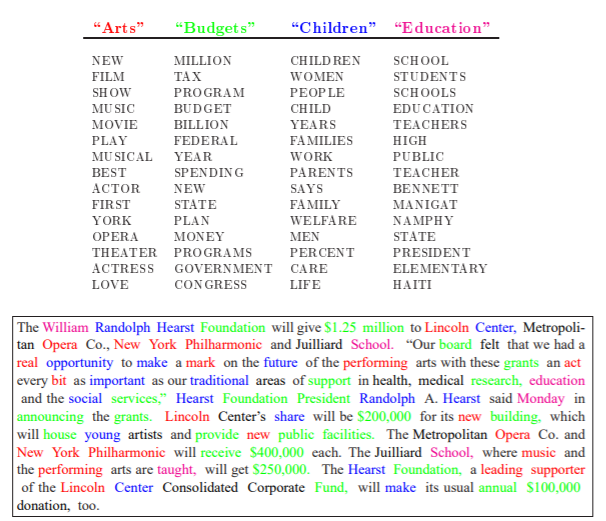
Note: Exemplary illustration of findings from an LDA on a corpus of news articles. Topics are mixtures of words. Documents are mixtures of topics. Source: Blei, Ng, Jordan (2003)
10.3.13 Topic Modeling: Latent Dirichlet Allocation (2)
- specify number of topics (k)
- each word (w) in each document (d) is randomly assigned to one topic (assignment involves a Dirichlet distribution)
- these topic assignments for each word w are then updated in an iterative fashion (Gibbs Sampler)
- namely: again, for each word in each document two probabilities are repeatedly calculated:
- “document”-level: proportion of words in document d belonging to a certain topic t (beta) (relative importance of topics in documents)
- “word”-level: proportion of words being assigned to a certain topic t in all other documents (gamma) (relative importance of words in topics)
- each word is reassigned to a new topic which is chosen as the probability of p = beta x gamma (overall probability that a certain topic generated the respective word w, put differently: overall probability that that w belongs to topic 1, 2, 3 or 4 (if k was set to 4)
- Assignment stops after user-specified threshold, or when iterations begin to have little impact on the probabilities assigned to words in the corpus
10.3.14 Topic Modeling: Structural Topic Models (vs. LDA)
- Structural Topic Models (short: STM) employ main ideas of LDA but add a couple more features on top
- e.g., STM recognizes if topics might be related to one another
- e.g., if document 1 contains topic A it might be very likely that it also contains topic B, but not topic C, i.e., main aspect of a Correlated Topic Model
- LDA assumes uncorrelated topics
- especially useful for social scientists who are interested in modeling effects of covariates (e.g., year, author, sociodemographics, time)
- documents with similar values on covariates will tend to be about the same topics
- documents with similar values on covariates will tend to use similar words/vocabulary to describe the the same topic
- by allowing to include such metadata, STM exceeds a simple bag-of-words approach
- LDA assumes stationary distribution of words within a topic (e.g., topic 1 for document 1 uses identical terms as topic 1 for document 2)
- spectral initialization (produces the same result within a machine for a given version of stm without setting a seed)
- additional R package (stminsights) provides strong focus on diagnostics etc.
- blogpost on detailed explanation of differences between LDA and STM
- e.g., STM recognizes if topics might be related to one another